Experiments on Hyperparameter tuning in deep learning — Rules to follow

Credits — https://image.freepik.com/free-photo/gear-cutting-machine_137573-2479.jpg

Any Deep Learning model has a set of parameters and hyper-parameters. Parameters are the weights of the model. These are the ones that are updated at every back-propagation step using an optimization algorithm like gradient descent. Hyper-parameters are set by us. They decide the structure of the model and the learning strategy. For example — batch size, learning rate, weight decay coefficient (L2 regularization), number and width of hidden layers and many more. Because of the flexibility deep learning provides in model creation, one has to pick these hyper-parameters carefully to achieve the best performance.

In this blog, we discuss

1. General rules to follow while tuning these hyper-parameters.

2. Experiment results on a data-set to verify these rules.

Experiment Details

Dataset

Hardware —

NVIDIA 1060 6GB GPU.

2. For experiments on batch size, kernel width, weight decay — Custom architecture (see code).

2. Test accuracy at each epoch

3. Average time for each epoch (train and inference on the test set)

Hyper-parameters and their effect on model training

We take an example of a Convolutional Neural Network (CNN) to relate model behavior and hyper-parameter values. For this post, we discuss the following — Learning rate, batch size, kernel width, weight decay coefficient. But before we discuss these general rules, let’s revisit our goal for any learning algorithm. Our goal is to reduce train error AND the gap between train error and test/validation error . We achieve this by tuning the hyper-parameters

A general plot for train and validation error. Original image.

Let’s look at how deep learning literature describes the expected effect of changing hyper-parameter values

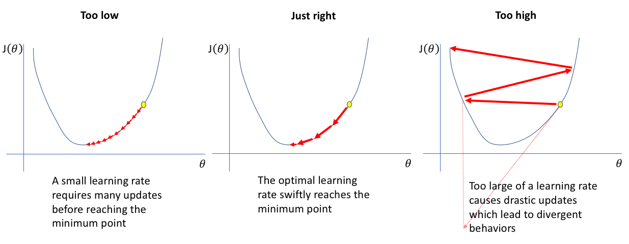
Learning Rate

The Deep Learning book says —

If you have time to only tune one hyper-parameter, tune the learning rate

In my experiments, this certainly holds. After trying three learning rates, I found that too low or too high value heavily degrades the performance of the algorithm. For a learning rate 10^-5, we achieve a test accuracy of 92% For the rest two rates, we barely cross 70% All other hyper-parameters are kept constant.

Test accuracy on ResNet

If you look at the error plots, there’s something to observe. For example in the training error —

Train Error on ResNet

As expected, all three decrease. But at the lowest learning rate (in pink), the loss at the 10th epoch is greater than the loss for the red curve at the first epoch . With extremely low learning rates, your model learns real slow. Also, at high learning rates, we expect the model to learn faster. But as you can see, the lowest train error on the red curve is still greater than the error on the orange curve (moderate learning rate). Now let’s look at the test error —

Test Error on ResNet

A couple of observations. For the lowest rate, the test loss decreases steadily and doesn’t seem to have reached the lowest point yet. Meaning the model has under-fit and perhaps needs more training.

image credits — https://www.jeremyjordan.me/content/images/2018/02/Screen-Shot-2018-02-24-at-11.47.09-AM.png

The red curve shows unusual behavior. One may suspect that due to the high learning rate, the optimizer couldn’t converge to a global minima and kept bouncing on the error landscape.

For the moderate curve (orange), the test error starts to increase slowly after the first epoch. This is a classic example of overfitting .

Batch Size

If you are familiar with Deep Learning, you must have heard of Stochastic Gradient Descent (SGD) and batch gradient descent. To revisit, SGD performs a weight update step for each data-point. batch performs an update after averaging gradients from the data-point in the entire training set. According to Yann LeCun

Advantages of SGD —

1. Learning is much faster

2. Often achieves a better solution

3. Useful for tracking changes.

Advantages of batch learning —

1. Conditions of convergence are well understood.

2. Many accelerated learning techniques like conjugate gradients are well understood in batch learning.

3. Theoretical analysis of weight dynamics and convergence rates are much simpler

Using a method somewhere in between, mini-batch gradient descent is popular. Instead of using the entire training set to average the gradients, average over gradient of a small fraction of data-points is used. The size of this batch is a hyper-parameter.

To illustrate, consider the loss landscape as shown in the figure below

Example loss landscape. Original picture

The diagonal lines with numbers on them are loss contours. The x and y-axis are two parameters (say w1 and w2 ). Along a contour, the loss is constant. For example, for any w1 and w2 pair lying on a line with loss 4.500, the loss is 4.500. The blue zig-zag line is how an SGD would behave. The orange line is how you expect a mini-batch gradient descent to work. The red dot represents the optimal value of the parameters, where the loss is minimum.

The book Deep Learning provides a nice analogy to understand why too-large batches aren’t efficient. The standard error estimated from n samples is σ/√ n. Consider two cases — one with 100 and another one with 10000 examples. The latter requires 100 times more computation. But the expected reduction in standard error is just by a factor of 10

In my experiment, I changed the batch-size. The test accuracy I obtained looked like —

Kernel Width

Convolution operation in CNN’s involves a kernel extracting features from a feature map. The kernel is made up of learned parameters. In 2-D convolutions, a kernel is an N*N grid, where N is the kernel width.

Increasing or decreasing the kernel width has its pros and cons. Increasing the kernel width increases the parameters in the model, which is an obvious way to increase the capacity of the model. It’s hard to comment on the memory consumption because the increased number of parameters increases the memory usage, but the output dimensions of the feature maps are smaller which decreases the memory usage.

Weight decay

Weight decay is the strength of L2 regularization. It essentially penalizes large values of weights in the model. Setting the right strength can improve the model’s ability to generalize and reduce overfitting. But a value too high will lead to severe underfitting. For example, I tried a normal and extremely high value of weight decay. As you can see, the learning capacity is almost none when this coefficient is set poorly.

Conclusion

The experiments fairly confirmed most of our hypotheses. A poorly tuned complex model like ResNet18 can easily perform worse than a well-tuned simple architecture. The loss curve is a good starting point to investigate the impact of hyper-parameters