

Frink
source link: https://futureboy.us/frinkdocs/
Go to the source link to view the article. You can view the picture content, updated content and better typesetting reading experience. If the link is broken, please click the button below to view the snapshot at that time.
About Frink
Frink is a practical calculating tool and programming language designed to make physical calculations simple, to help ensure that answers come out right, and to make a tool that's really useful in the real world. It tracks units of measure (feet, meters, kilograms, watts, etc.) through all calculations, allowing you to mix units of measure transparently, and helps you easily verify that your answers make sense. It also contains a largedata file of physical quantities, freeing you from having to look them up, and freeing you to make effortless calculations without getting bogged down in the mechanics.
Perhaps you'll get the best idea of what Frink can do if you skip down to thefurther on this document. Come back up to the top when you're done.
Frink was named after one of my personal heroes, and great scientists of our time, the brilliant Professor John Frink. Professor Frink noted, decades ago:
"I predict that within 100 years, computers will be twice as powerful, ten thousand times larger, and so expensive that only the five richest kings of Europe will own them."
Features
For those with a short attention span like me, here are some of the features of Frink.
- Tracks units of measure(feet, meters, tons, dollars, watts, etc.) through all calculations and allows you to add, subtract, multiply, and divide them effortlessly, and makes sure the answer comes out correct, even if you mix units like gallons and liters.
- Arbitrary-precision math, including huge integers and floating-point numbers, rational numbers (that is, fractions like 1/3 are kept without loss of precision,) complex numbers, and intervals.
- Advanced mathematical functionsincluding trigonometric functions (even for complex numbers,)factoring and primality testing, and.
- between thousands of unit types with a huge built-indata file.
- (add offsets to dates, find out intervals between times,) timezone conversions, and user-modifiable date formats.
- between several human languages, including English, French, German, Spanish, Portuguese, Dutch, Korean, Japanese, Russian, Chinese, Swedish, and Arabic.
- Calculatesbetween most of the world's currencies.
- Supportsthroughout, allowing processing of almost all of the world's languages.
- Supports(also known as Interval Computations ) in calculations, allowing you to automagically calculate error bounds and uncertainties in all of your calculations.
- ReadsHTTP and FTP-based URLsas easily as reading local files, allowing fetching of live web-based data.
- Runs on most major operating systems (anything with Java 1.1 or later,) as anapplet, through aweb-based interface, onAndroid, and onmany mobile phones and hand-held devices.
- Installs itself on your system in seconds usingand automatically keeps itself updated when new versions of Frink are released.
- Runs with aGraphical User Interface(Swing, AWT, andAndroid) or a command-line interface.
- User interface has awhich allows you to write, edit, save, and run extremely powerful programs even on a handheld device.
- Frink has a simple but powerful system for drawingwhich are resizable, support transparency and anti-aliasing, and can be printed or written to image files. Graphics can also have exact lengths, so that a 3-centimeter line is three centimeters long when printed.
- PowersFrink Server Pages, a system for providing dynamic web pages powered by Frink.
- Frink allowsObject-Oriented Programming, which allows you to create complex data structures that are still easy to use.
- layer allows you to call any Java code from within Frink.
- Frink can also beembedded in a Java program, giving your Java programs all the power of Frink.
Get Notified
Frink changes almost every day. If your version of Frink is more than a few days old, you're probably out of date! The latest versions are always available here. Keep an eye on theWhat's New page to see new features and keep abreast of its rapid developments.
While that page is the most detailed and constantly-updated source of information about changes in Frink, I also announce new features on Twitter at @frinklang . And if you want to follow Alan's personal ramblings for some reason, those are at @aeliasen .
Donate
If you find Frink useful, there are lots of ways you can donate to its further development. I'd really appreciate it!
Mailing Lists
General Frink list (low-traffic):
To receive periodic notifications of general interest about the Frink language, please join the Frink mailing list . (Hosted by Yahoo! Groups. Link opens in new window.) This is a lower-traffic list, mostly for announcements.
Detailed Frink list (higher-traffic):
For detailed discussions about particular programs, programming help, algorithms, and details of the Frink language, please join the Frink-discuss mailing list . (Hosted by Yahoo! Groups. Link opens in new window.) This is the appropriate place for posting programming questions and will probably be a higher-traffic list.
OoooOoo Frink Science:
This list is intended to discuss problems in math, science, and physics and explore solutions using the Frink language.
Frink Science mailing list . (Hosted by Yahoo! Groups. Link opens in new window.)
Presentations and Papers
You can read (and watch using RealPlayer) my presentation Frink -- A Language for Understanding the Physical World that I gave on Frink at the Lightweight Languages 4 conference at MIT. This discusses some of the design decisions of Frink, how it has evolved, implementation details, and future directions for the language.
Table of Contents
- Experimental Versions
- How Frink is Different
- Setting Display Units
- Setting Number Formats
-
- Security Restrictions on eval[]
-
- Initializing OrderedList
-
- Making Interactive Interfaces
-
- Dictionary Constructors
-
- Unicode Character Codes
- Correct String Parsing
- Other String Functions
- Defining New Date/Time Formats
-
-
Regular
Expression Reference
- Basic Patterns and Metacharacters
- Special Character Classes
- Unicode Character Classes
- Pattern Match Modifiers
-
Regular
Expression Reference
-
- Substitution with Expressions
- Including Other Files
- Object-Oriented Programming
-
- Introduction to Graphics
-
- Polygons and Polylines
- Transforming Graphics
-
- Drawing images into graphics
- Sample Graphics Programs
-
- Historical U.S. Price Data
- Historical British Price Data
- International Exchange Rates
-
- Interval Arithmetic Example
- Interval Comparison Operators
- Interval Arithmetic Status
-
- Creating Java Objects
- Calling Static Java Methods
- Accessing Static Java Fields
- Calling Functions and Methods by Name
- Iterating Over Java Collections
-
- Sniping eBay Auctions
- Why is Superman so Lazy?
- Saving Hundreds of Millions of Dollars
Using Frink
Try as you read
If you want to try the calculations as you're reading, click here to open the web-based interface in a new window. The web-based interface gives hints for new users, which may make it the easiest way to learn how to use Frink.
If you have a frames-enabled browser, and you don't see a Frink sidebar to the left, you can also click here to try Frink in a sidebar as you read this. (The sidebar mode doesn't give as many hints, though.)
Download using Java Web Start
Quick Start:
On many platforms, if you already have Java installed,
you can start Frink in the GUI mode by simply downloading and
double-clicking the
frink.jar
file. For more
startup options, see thesection.
Another method of installation requires Java Web Start, which is installed with most versions of Java. Using Java Web Start
is used to be a great way to run Frink if you don't need to run programs from the command-line. (But you can still write and run programs from the GUI using Java Web Start!) If you do want to run programs from the command-line, see thesection below. Java Web Start will allow you to automatically get the latest version of Frink and will update Frink automatically when new versions are available.
Installation Steps
- If you don't have a recent version of Java, you can get it from Sun. (Link opens in new window.)
- ( Optional ) If you've never installed anything with Java Web Start, please read and understand the FAQ entry about the security warnings you'll see (link opens in new window) and your alternate download options.
-
Warning:
Most major browsers have now disallowed Java plugins to run in the browser. However, if you have a Java Virtual Machine installed, you probably still have Java Web Start installed, which you need to invoke from the command-line with the command
javaws. In Fedora, you can make sure this is installed by installing theicedtea-webpackage from your package manager, e.g. as root, typingdnf install icedtea-weband then one of the commands below. In Debian-like environments, you may install this by installing theicedtea-netxpackage, e.g. as root, typingapt-get install icedtea-netxand then one of the commands below. -
Warning:
If you're using Java version 7u51 or later, they silently and incompatibly decided to change default security settings so you'll need to open the Java Control Panel to allow Frink to run. Otherwise you will see a dialog that says something like "Application blocked by security settings" or "Your security settings have blocked a self-signed application from running." (This silent change was made after 12+ years of the aforementioned method working fine.)
The best way to allow Frink to run is to follow the instructions listed here and add
http://futureboy.usto the exceptions list in step 7.Note: As always, Java's instructions and installer are terrible, and the Java Control panel on Windows may actually be under your Start menu as
Java|Configure Java, or under your Windows Control Panel, or if you start your Control Panel and don't see it, Java's control panel will be hidden under "32-bit Control Panel." And sometimes you'll have multiple versions of Java installed and the one that gets started isn't the latest version. I had lots of problems until I manually uninstalled all the versions of Java on the Windows machine, reinstalled the latest version, and uninstalled Frink and reinstalled it. Sorry about that. Windows and Java integration is terrible. (Theicedtea-webpackage for Fedora and other installations contains a vastly better implementation of Java Web Start.) -
Click one of the options below to install Frink: (see the screenshots below):
-
Swing Interface
Prettier. Requires Java 1.5.0 or later.
Note: If your browser no longer supports Java in the browser, you can probably install this from the command-line by typing:
javaws https://futureboy.us/frinkjar/frink.jnlp -
Swing Interface with standard
libraries
. This is a version of Frink that contains a variety of standard libraries
and useful programs. It's a larger download, but the standard libraries change somewhat infrequently and should only get downloaded when changes are made.
Note: If your browser no longer supports Java in the browser, you can probably install this from the command-line by typing:
javaws https://futureboy.us/frinkjar/frinkwithlibs.jnlp -
AWT Interface
- Not as pretty as the Swing mode, but will run on older JVMs.
Note: If your browser no longer supports Java in the browser, you can probably install this from the command-line by typing:
javaws https://futureboy.us/frinkjar/frinkawt.jnlp
-
Swing Interface
If you've read thosesecurity notes, and understood what the security messages are telling you, and the warnings are still too scary, (and you don't want to send me the $400 per year it would cost me to remove at least one of them,) and you'd rather download a limited version of Frink that runs in the most restrictive security sandbox (breaking some features), then click here to install a limited version of Frink. Again, please read thosesecurity notes to see what features will be unavailable if you choose this option. You can always get the full version of Frink later if you need those features.
If someone wants to send me the $400 necessary to get a VeriSign "Code Signing Cerificate", I'll sign it just for you. It won't work any differently.)
If you have an old version of Java Web Start, Frink will probably show up
in the "Downloaded Applications" section of the Java Web Start panel which
isn't immediately visible. Use the View
menu option to select
the Downloaded Applications tab. It will also let you create a Frink
shortcut on your desktop or in your start menu. The defaults in Java Web
Start before version 1.4.2 are set oddly so that the second
time
you run Frink, it will ask you if you want to make a shortcut.
If you're using Linux, and Sun's Java release, only Java version 1.5 beta and later will install shortcuts onto your desktop and start menu. Highly recommended.
User Interface Options
Swing User Interface
The Swing version allows mixed fonts and colors. Due to some performance bugs in Sun's Swing implementation (like large paragraphs taking several minutes to paint every time you resize or scroll,) it can be problematic. As of 2008-08-25, the capabilities of the Swing and AWT interfaces are about the same.
AWT User Interface
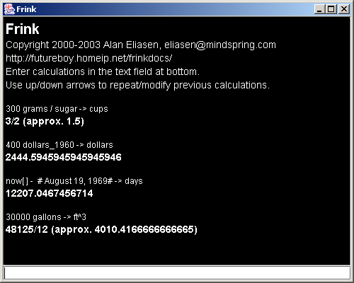
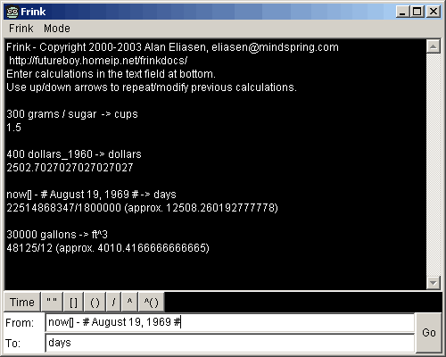
The AWT user interface has several modes. The two-line conversion mode andare shown below. Small devices usually can't run Swing, but all Java platforms should be able to run AWT.
Frink As An Applet
If your web browser supports Java 1.3.1 or later, try the Java Applet-based interface . It looks and works just like the GUI above, but it requires you to be connected to the internet and must download for each session.
Your browser must support Java 1.3.1 or later, or you will need to get download a newer version of Java from Sun. It is extremely highly recommended that you have Java 1.5.0 update 2 or later. This has been tested with Internet Explorer, Netscape 4.x, Netscape 6+, Mozilla (Windows and Linux), and Opera.
If you don't have a recent version of Java, you can get it from Sun. (Link opens in new window.)
(The certificate is just signed by me, so you'll get a warning. Network access is necessary to use the network portions of Frink... like currency calculations, translations, etc. If you deny network access, the non-network parts of Frink will work just fine. If someone wants to send me the $400 necessary to get a VeriSign "Code Signing Cerificate", I'll sign it just for you. It won't work any differently.)
Web Interface
If the applet doesn't work for you, try theweb interface. It should allow you to use the latest version of the Frink engine. It is now powered byFrink Server Pages.
In this web interface, you can enter any Frink expression in the "From:"
box. If you also enter a value in the "To:" box, it is treated as the
right-hand side of a conversion expression (that is, to the right of the
conversion operator ->
)
Thus, to convert 10 meters to feet, you can enter 10 meters
in the "From" box and feet
in the "To" box, or, equivalently, type 10 meters -> feet
in the
"From" box and leave the "To" box empty. It does exactly the same thing.
Downloading Frink
Quick Start:
On many platforms, if you already have Java installed,
you can start Frink in the GUI mode by simply downloading and
double-clicking the
frink.jar
file.
If you're just using Frink for interactive calculations, or are happy using the built-in programming mode and you're not writing running programs from the command-line, see thesection above.
(If you're looking for an installer for handheld devices, like Android, see thesection below.)
If you want to write full Frink programs and
run them from
the commmand-line, you will need to get your own copy of Frink, and
have a Java 1.1 or later runtime environment on your machine,
1.4.2+ is recommended as it's less buggy. The date calculations in
anything before Java 1.3 are rather bad,) you may download the
latest executable jar
file. (Note that this changes
almost daily as I do more work, so download often.)
Otherwise, here are the steps to downloading Frink:
- If you don't have a recent version of Java, you can get it from Sun. (Link opens in new window.)
- Download frink.jar .
- (Double-clicking the file you just downloaded might start Frink in GUI mode, depending on your operating system. If that's not enough, read on.)
- See thesection below for directions for starting full Frink programs, running from the command-line, etc.
Running Frink
Quick Start:
On many platforms, if you already have Java installed,
you can start Frink in the GUI mode by simply downloading and
double-clicking the
frink.jar
file.
If you want to run Frink in command-line mode, here are a couple of sample scripts you can use to start Frink. You will need to edit them to match the paths on your system!
In the samples below, you may need to replace java
or javaw
with the full path to your Java Virtual Machine,
whatever that may be. Note that javaw
is a Windows-only
command that simply starts Java without opening a console window. You'll
probably replace this with java
on other platforms.
The most general way to start Frink is to launch the frink.gui.FrinkStarter
class:
java -cp frink.jar frink.gui.FrinkStarter
    [options]
(The above starter scripts use this class. Look at them first.) By default, this starts in text mode but allows many command-line options to start in different modes:
Switch Description --swing Starts in Swing GUI mode --gui Starts in Swing GUI mode --awt Starts in AWT GUI mode --fullscreen Starts fullscreen --prog Starts in programming mode with a blank program -open filename Starts the specified filename in programming mode (this option is passed by double-clicking a file in Windows if you have file associations set up.)Other start options are listed below, if you want to use them. I'd suggest using one of the scripts above and modifying it.
To run the jar file in text mode (only), use:
java -cp frink.jar frink.parser.Frink [options]
To run the jar file with the Swing GUI, (shown above under,) use:
javaw -cp frink.jar frink.gui.SwingInteractivePanel [options]
The Swing GUI is the default action for the jar file, so this is the same as saying:
javaw -jar frink.jar [options]
To run the jar file with the AWT GUI, which gives access to several modes, including programming mode, use:
javaw -cp frink.jar frink.gui.InteractivePanel
    [options]
To run the jar file and start the AWT GUI in programming mode, use:
javaw -cp frink.jar frink.gui.ProgrammingPanel
    [filename]
To run the jar file and start the Swing GUI in programming mode, use:
javaw -cp frink.jar frink.gui.SwingProgrammingPanel
    [filename]
If a single filename is specified in programming mode, this file will be loaded into the interface.
To run the AWT GUI in full-screen size (this is primarily for small devices,) use:
javaw -cp frink.jar frink.gui.FullScreenAWTStarter
    [options]
Depending on your operating system, I recommend that you write a shell script, batch file, or create a shortcut to let you run this even more easily (see below for samples.) To exit, use Ctrl-C, or send your platform's end-of-file character (usually Ctrl-Z or Ctrl-D), possibly followed by carriage return. Or just close the window.
See thebelow for additional options if you're running behind a HTTP or FTP proxy server.
Also see thesection below to see how to improve speed.
Command-Line Options
Arguments passed in on the command-line are treated as names of Frink programs to be executed. Other command-line options are listed below.
If you just want to have Frink calculate something and exit, you can pass
arguments on the command line using the -e [string]
switch. Each command-line argument following the -e will be interpreted as
a Frink expression, making it easy to run Frink from other applications:
java -cp frink.jar frink.parser.Frink -e "78 yards -> feet"
234.0
Other command-line options:
Switch Description -f filename Allows you to specify multiple Frink source files to load and run. Multiple-f filename
options may be specified. If this option is specified, the specified file will not
receive any following command-line arguments.
The -f
switch is no longer required or recommended unless you are loading multiple files.
Normally, you will just specify the filename to load as the last command-line argument.
For example, to load your own definitions from mydefs.frink
before loading the main program main.frink
, you may do something like:
frink -f mydefs.frink main.frink args
.jar
file) and modify it to suit your needs.
--nounits -nu Don't load a units file at all on startup. This will improve startup time, but will break all programs that use any of the standard units. No units of measure will be defined at all. -I path Appends the specified path to the paths that will be searched when a
use
statement is encountered in a program. This may be either an absolute or relative file path. You may specify multiple -I
arguments on the command-line, and the paths will be searched in the order they are specified.
--encoding str
Specify the character encoding of all following Frink program files. This option must precede the filename that it modifies.
Frink programs can now be more directly written in any language and encoding system. This switch is only necessary if your system's default encoding (as detected by Java) is different than that of the program file you're loading.
The encoding is a string representing any encoding that your version of
Java supports, e.g.
"UTF-8"
, "US-ASCII"
, "ISO-8859-1"
, "UTF-16"
, "UTF-16BE"
, "UTF-16LE"
. Your release of Java may support more
charsets, but all implementations of Java are required to support the
above. The sample programencodings.frink also demonstrates how to list all of the encodings available on your system (and
their aliases.)
If you specify multiple files having different encodings using multiple -f
directives, you can use something like --encoding ""
to set the encoding back to your
system's default.
This flag does not
alter the behavior of files opened using
commands like read[]
or lines[]
. To change
their behavior, use thetwo-argument versions of these
commands.
-v
--version
Print out the Frink version and exit. (From inside a program, you can call the function FrinkVersion[]
to return the current version.)
--sandbox
Enables Frink's internal "sandbox" mode so you can run untrusted code. This is different from Java's sandbox, in that it enables only Frink's notions of what should and shouldn't be allowed. It disallows programs to define functions and many other things, so it's rarely useful to the end-user, and hardly any programs will run this way. It's really more for my testing.
--ignore-errors
Ignores syntax errors when parsing a program and attempts to ignore those lines and recover and run the program. Generally a very bad idea, but this flag was added to preserve old, excessively-permissive behavior.
Handling Command-Line Arguments
Any command-line arguments after the name of the program to be executed
are passed to the program as ancalled ARGS
.
Experimental Versions
For those who want a standalone, all-in-one Frink download, there is an experimental, unsupported version of Frink compiled for Windows only using an experimental, unreleased version of the GNU compiler for Java (GCJ). This only works in command-line mode, but requires no other downloads and may start up more quickly. It is appropriate for quick calculations and command-line scripts. Not all functions may work. Let me know about parts that do or don't work for you. It is compressed with UPX to reduce the file size (possibly at the cost of some startup time.) This version starts up more quickly than the Sun JVM, but runs programs about 5-6 times slower.
- Experimental, Unsupported executable for Windows:frinkx.exe.
(Unfortunately, it's compiled without optimization, because that pegs the CPU for over 72 minutes, and then blows out my system after trying to use over a gigabyte of virtual memory. Anyone want to donate me a new computer with tons of memory? Or try compiling it with -O3?) For Windows, you can use this experimental gcj 4.3 eclipse-merge-branch version.
Hint: If you install the gcj package linked above, or have a working GCJ (4.3 or later is required) for other platforms, the command line to compile with full optimization will be something like:
gcj -O3 -fomit-frame-pointer --main=frink.parser.Frink -o frinkx.exe frink.jar
Small Devices
Frink can run entirely on handheld devices like the any phone running the Android platform, Sony Ericcson P800, P802, or P900 smartphone, the Nokia 92x0 Communicator (Nokia 9210, 9210i, and 9290), and the Sharp Zaurus.
The installer is built as part of the Frink release process, so these versions will be up-to-date with the latest Frink. (The version numbers in the installers may not change, though.)
Download the installer for the following platforms:
- Android - All of Frink's functionality, including graphics, is available on the Android mobile phone platform. See theFrink on Android page for more information on using Frink on Android. As Android is a stable, complete, widely-available, well-designed, multi-platform and multi-vendor environment, it will probably be the primary platform for Frink on handheld devices in the future. Other proprietary platforms that require extensive porting and packaging for every phone model may go away.
- Sony Ericsson P800, P802 or P900, and Motorola A920 or A925 (and perhaps other Symbian 7.0 devices with the UIQ2 user interface.)
- Nokia Communicator 92xx (Nokia 9210, 9210i, and 9290) (and perhaps other Symbian 6.0 devices with the "Crystal" (wide-screen) user interface). You need 3 to 4 megabytes of free memory to run Frink.
-
Sharp Zaurus
(despite the filename, this isn't ARM-processor specific--it's pure Java, and might work on other platforms that use the
.ipkpackage format.) Note: I need help testing and improving this installation package. Please contact Alan Eliasen if you have experience with Zaurus installer packages. Hint for helpers: an.ipkfile is just a.tar.gzfile, so you can open it up and poke around, but I don't have a Zaurus to test on. -
Experimental:
Nokia 9300,
Nokia 9500 Communicator
(and perhaps other Symbian Series 80 devices.) I need help testing this one. The Series 80 devices evidently crash when you try to add menubars, so some functions are impossible to access. This is a jar file customized for Series 80, and not an
.sisinstaller.
Notes about running Frink on other devices, including notes about why I probably won't provide releases for newer Symbian devices that require their "Symbian Signed" abomination, please seethis FAQ entry.
If you have problems running any of these, please contact Alan Eliasen . Since I don't own any of these devices, I rely on others for testing and detailed bug reports. (The emulators don't always work like the real devices!) It's possible for bugs to slip in that work under normal testing, but cause problems on the limited/different JVMs on these devices.
If anyone knows of a Symbian 6.0 device with the "Quartz" user interface that supports PersonalJava, please let me know and I can give you an installer to test.
If you know of a device that supports PersonalJava 1.1 or better, including
the java.math
package and floating-point math, and you think
Frink would run on this device and you would like to help test it, please suggest it to me.
.
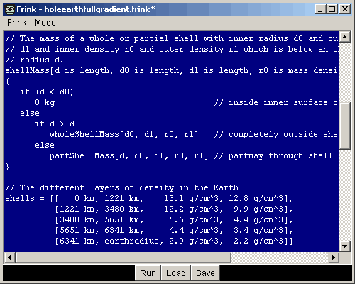
Programming Mode
If you want a unified environment to write, run, save, and load Frink
programs, try the programming mode. You can either start this mode
explicitly (see thesection
below) or, from the AWT GUI, choose the menu option Mode |
Programming
.
This mode is primarily designed to allow programming on small devices, but can run on any platform.
The Data
menu option allows you to choose between thestandard data file and an alternate data
file. You'll usually want to use the standard data file, but on small
devices, it can take a long time to start your program, and may use a fair
amount of memory. The standard data file is big. In that case, you may
want to make a pared-down (or even empty) units file and use that when
running your programs.
For now, selecting a different data file is not a persistent setting. This setting will only remain in place until you exit Frink.
GUI Options
You can specify the width or the height of the window for frink.gui.InteractivePanel
or frink.gui.SwingInteractivePanel
or frink.gui.FullScreenAWTStarter
.
You may specify width or height or both. For example:
java -cp frink.jar frink.gui.SwingInteractivePanel
    --width 500 --height 400
Performance Tips
There are several things you can do to make your Java Virtual Machine (JVM) run Frink more quickly:
- Java 8 contains my algorithmic improvements to make large integers work much more quickly for multiplication, base conversion, etc. (It only took the Java people 11+ years to import my patches.)
-
For long-running programs, if you're using Sun's Java Virtual Machine (JVM), use the
-servercommand-line switch to thejavaexecutable. This starts the Server VM which optimizes more aggressively and often improves performance of long-running programs by a factor of 2, but at the expense of increased start-up time. Note that the server VM may not be available if you just downloaded the Java Runtime Environment (JRE), and not the full Java Software Development Kit (SDK). - If you're not starting long-running programs, and want the fastest start-up time, don't use the Server VM.
-
Like all Java programs, Frink can often run much faster if you allow the JVM to use more memory at startup, leading to less-frequent garbage collection. In Sun's implementation, this is achieved by passing the options
-Xmx<size>(for maximum Java heap size) and-Xms<size>(for initial Java heap size) to thejavaexecutable. The size arguments are something like256Mfor 256 megabytes. Note that this is at the expense of other processes running on your system, and should be used sparingly because allocating too much memory may cause your system to swap excessively or run out of memory if set too high. -
( Probably obsolete
) If you're doing mostly large integer work (factoring, primality testing, other number theory,) where most of the runtime is spent in mathematical operations on very large integers, the Kaffe
Virtual Machine compiled with the incredibly fast GMP
numerical libraries works literally thousands of times faster than Sun's VM and its horribly naïve algorithms.
Warning: Make sure that GMP is compiled with the configure option
--enable-alloca=malloc-reentrantor you'll blow out the stack and crash with very large integers.Warning: As of the 2004-07-18 release of Kaffe, you must now explicitly pass the
-Xnative-big-mathargument when running Kaffe in order to use the GMP libraries.
Proxy Configuration
If you use a HTTP or FTP proxy server, you need to add some options to your
command lines (say, right after the word java
) to use the
proxy if you want certain functions to work. HTTP and FTP are used for the
following:
- Language translations(HTTP)
- Currency/Exchange Rate conversions(HTTP, will fall back to static file if unavailable)
- Historical values of the U.S. dollar(FTP, will fall back to static file if unavailable)
The following are settings for Sun's distribution of Java 1.4.1. You may need different options depending on your Java distribution. See Sun's Networking Properties documentation for more properties you may need if you're on a network that requires more proxy settings.
HTTP proxy:
-Dhttp.proxyHost=proxyname
    -Dhttp.proxyPort=portnum
FTP proxy:
-Dftp.proxyHost=proxyname
    -Dftp.proxyPort=portnum
These settings should not be necessary when using the applet version or the Java Web Start version, as these inherit the proxy settings from your browser or the Java Web Start Application Manager respectively.
How Frink is Different
Frink is, first and foremost, designed to make it easy to figure out things. If there's a unifying principle in Frink, it could be considered to be the normalization of information . I'm trying to simplify and unify the representation of data so that you can perform all sorts of interesting operations on them. Whatever that means.
Frink is optimized for doing quick, off-the-cuff calculations with a minimum of typing, primarily so it can be used with handheld devices which can make text entry difficult (especially symbols). This doesn't mean that Frink is unsuitable for doing large, very high accuracy calculations. It does those well, too, and the complicated calculations look just like the simple ones.
To give an example, Frink represents all numerical quantities as not simply a number, but a number and the units of measurement that quantity represents. So you can enter things such as "3 feet" or "40 acres" or "4 tons", and add, subtract, multiply, etc. these things together. Frink will track the resulting quantities through all calculations, eliminating a large category of errors. You can add feet, meters, or rods all in the same calculation and the details are handled transparently and correctly.
It also knows the ways that these units are interrelated-- a length times a length is an area; length 3 is a volume (if you believe in the hypothetical Z axis); mass times distance times acceleration is energy. If you know something in one system of measurement you can convert it to any other system of measurement.
All units are standardized and normalized into combinations a small number of several "Fundamental Dimensions" that cannot be reduced any further. These are completely arbitrary and configurable but are currently:
Quantity Fundamental Unit Name length m meter mass kg kilogram time s second current A ampere luminous_intensity cd candela substance mol mole temperature K Kelvin information bit bit currency USD U.S. dollarLook at thedata file for these definitions (and my editorializing on the boneheadedness of many these choices.) The data file recursively defines all measurements in terms of the fundamental units.
An exponent can be attached to each dimension. For example, an area is
length * length which might be represented as meters^2
. Of
course, a negative exponent indicates division
by that quantity,
so meters/second will be displayed as m s^-1
, or acceleration
(which can be represented as meters per second per second) is represented
as m s^-2
.
Numeric Types
Numeric values in Frink are represented in one of three ways:
Integer An arbitrarily large number with no decimal part. Represented as a number with no decimal point, ( e.g.1000000000
) or the special "exact exponent" form 1ee9
. An integer can also contain underscores for better readability, e.g.
1_000_000_000
Rational
An arbitrarily large number which can be written as integer/integer ( such as 1/3
or 22/7
). Rational numbers are first reduced to smallest terms; that is, 2/10
is stored as 1/5
and 5/5
is stored as the integer 1
Floating Point
1.
or 1.01132
, as well as any approximate exponential such as 2e10
or 6.02e23
.
As of the 2018-12-11 release, if a rational number has the "exact
exponent" indicator ee
, it is turned into an exact rational
number or integer. For example, the new exact SI value for Avogadro's
number 6.02214076ee23
will become an exact integer. The
exponents can also be negative, which will usually lead to an exact
rational number, such as 6ee-1
which produces the exact
rational number 3/5 (exactly 0.6)
.
i
. For example, 40 + 3 i
. The real and imaginary parts of a complex number can be any of the numerical types listed above.
Intervals
An interval represents a range of values, such as [2.1, 3] where, depending on your interpretation, the actual number is unknown, but contained within this range, or the number simultaneously takes on all values within the range. See theInterval
Arithmeticsection of the documentation for more information.
Data Libraries
Frink knows about a wide variety of measurements. You can usually type a unit of measurement in a variety of ways. Plurals are usually understood. Case is important (and somewhat arbitrary until I do some normalization and cleanup of the units file, but usually lowercase is your best choice.) The following are all examples of valid units:
-
1 -
1000000 -
1_000_000(also one million, just maybe more readable.) -
1E6(1.0x10 6 , or approximately a million (floating-point)) -
1EE6(1x10 6 , or exactly a million (integer)) -
million -
1 million -
24.5E-10(24.5 x 10 -10 ) -
eighty -
four score + seven -
1(a dimensionless exact integer) -
1.0(a floating-point number) -
1.(also a floating-point number) -
1/3(a rational number, preserved as a fraction) -
1 quadrillion -
gallon -
1 gallon -
56 gallon -
56 gallons -
foot -
54.2 feet -
furlong -
hogshead -
2 USD("USD" is the ISO-4217 currency code for the U.S. Dollar) -
2 dollars(for now, shorthand for the U.S. dollar) -
16 tons -
6 ounces -
1 gram -
8 milligrams(most common prefixes are allowed.) -
8 mg(abbreviations of most prefixes and units are also allowed) -
7 kilowatts -
7 kW -
1.21 gigawatts -
1.21 GW -
9 seconds -
9 sec -
9 s -
1/24 day -
100001000101111111101101\\2(a number in base 2) -
1000_0100_0101_1111_1110_1101\\2(a number in base 2 with underscores for readability) -
845FED\\16(a number in base 16... bases from 2 to 36 are allowed) -
845fed\\16(a number in base 16) -
845_fed\\16(a number in base 16 with underscores for readability) -
0x845fed(Common hexadecimal notation) -
0x845FED(Common hexadecimal notation) -
0xFEED_FACE(Hexadecimal with underscores for readability) -
0b100001000101111111101101(Common binary notation) -
0b1000_0100_0101_1111_1110_1101(Binary with underscores for readability)
If you're looking for a specific unit, and don't know how it's spelled or capitalized, see thesection below.
Or, if you're using theweb interface, type part or all of the name in the "Lookup:" field and click "lookup". Selecting the "exact" checkbox will only return exact matches, otherwise you will get all lines containing that substring. Try it for something like "cubit" and you'll see that there are often lots of variations.
Important: You'll learn the most if you look at the voluminous and fascinatingdata file for more examples of things you can do, and measurements that Frink knows about.
Integrated Help
If you don't know the name of a unit or function, but can guess at it, you can either read thedata file for more information, or use the integrated help. Keep in mind that Frink is case-sensitive, so you'll need to use the right capitalization of the names.
Unit or function names can be looked up by preceding part or all of the name with a question mark. This will return a list of all units and function names containing that string, in upper- or lower-case. For example, to find the different types of cubits:
?cubit
[homericcubit, assyriancubit, egyptianshortcubit,
    greekcubit, shortgreekcubit, romancubit, persianroyalcubit, hebrewcubit,
    northerncubit, blackcubit, olympiccubit, egyptianroyalcubit,
    sumeriancubit, irishcubit, biblicalcubit, hashimicubit]
Or, if you want to know the name of the currency used in Iran,
?iran
[Iran_Rial, Iran_currency, Iran]
Simply enter the name of the unit you're interested in to see its value:
biblicalcubit
0.55372 m (length)
If you want to see the results in specific units of measurement, you
can use the arrow operator ->
as described in thesection below:
biblicalcubit -> inches
21.8
Or, if you want to see the sizes of all the units as a single unit type, and they're all the same, you can use the arrow operator on the list. The following sample shows all the different types of cubits the world has defined and converts them to inches:
?cubit -> inches
[homericcubit = 15.5625,

     assyriancubit = 21.6,

     egyptianshortcubit = 17.682857142857142857,

     greekcubit = 18.675,

     shortgreekcubit = 14.00625,

     romancubit = 2220/127 (approx. 17.480314960629922),

     persianroyalcubit = 25.2,

     hebrewcubit = 17.58,

     northerncubit = 26.6,

     blackcubit = 21.28,

     olympiccubit = 18.225,

     egyptianroyalcubit = 20.63,

     sumeriancubit = 2475/127 (approx. 19.488188976377952),

     irishcubit = 500000000/27777821 (approx. 17.99997199204358),

     biblicalcubit = 21.8,

     hashimicubit = 25.56]
If you don't want to see exact fractions, you can (as always) multiply the
right-hand-side by 1.0
or 1.
(without a zero
after the decimal point) to get approximate numbers:
?cubit -> 1.0 inches
If you use two question marks, the units that match that pattern will be displayed and their values in thecurrent display units:
??moon
    moonlum = 2500 m^-2 cd (illuminance),

    moondist = 0.002569555301823481845 au,

    moonmass = 73.483E+21 kg (mass),

    moonradius = 0.000011617812472864754024 au,

    moongravity = 1.62 m s^-2 (acceleration)
Note:
If you use the form with two question marks, you cannot
convert them to a specified unit with the ->
operator, as they have already been converted to a
single string.
Note: As of the 2016-07-06 release, the double-question-mark operator now returns a single string with newlines separating each entry, instead of a list of strings.
Note that functions are displayed at the end of the list, and can be distinguished from units by the square brackets following them:
??call
   callistodist = 1.883000000e+9 m (length),

   callistoradius = 2.400000e+6 m (length),

   callistomass = 1.08e+23 kg (mass),

   callJava[arg1,arg2,arg3]
In addition, the functions[]
function will produce a list of
all functions.
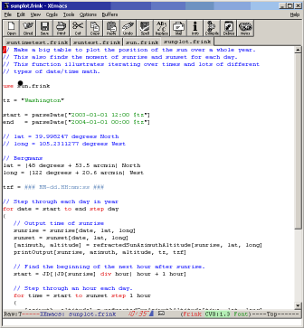
Editing Frink
If you're writing Frink programs, you can edit Frink files in your favorite text editor. If that happens to be Emacs or XEmacs, you can download the rudimentary Frink mode for Emacs . It's somewhat rough at this moment, but it has syntax highlighting, automatic indenting, ability to run interactive Frink sessions or programs. Screenshot is below.
Conversions
By default, the output is in terms of the "fundamental units". To convert
to whatever units you want, simply use the "arrow" operator ->
(that's a minus sign followed by a greater-than sign,)
with the target units on the right-hand side:
38 feet -> meters
11.5824
Formatting Shortcut: If the right-hand-side of the conversion is in double quotes, the conversion operator will both evaluate the value in quotes as a unit and append the quoted value to the result. So, the above example could be performed as:
38 feet -> "meters"
7239/625 (exactly 11.5824) meters
In this case, because the ratio between feet and meters is an
exactly-defined quantity, so the answer comes out as an exact rational
number. This is also displayed as a decimal number for your convenience.
If you just want the decimal value, you can multiply by an approximate
decimal number (any number containing a decimal point) such as 1.0
or 1.
without anything after the
decimal point:
38. feet -> "meters"
11.5824 meters
Note: If you are using the web-based interface, simply enter everything left of the arrow in the "From:" box and everything to the right of the arrow in the "To:" box. Or you can enter the whole expression including the arrow in the "From:" box and leave the "To:" box empty. It does the exact same thing.
If the units on either side of a conversion are not of the same type, Frink may try to help you by suggesting conversion factors:
55 mph -> yards
     Conformance error -

       Left side is: 15367/625 (exactly 24.5872) m s^-1 (velocity)

      Right side is: 1143/1250 (exactly 0.9144) m (length)

        Suggestion: multiply left side by time

                   or divide left side by
    frequency


     For help, type:

        units[time]

          or

        units[frequency]

        to list known units with these dimensions.
If you get an error like this, you can list all the units that have the
specified dimensions by typing units[time]
or units[frequency]
.
Yes, sometimes it gives digits which aren't significant in results. As I improve the symbolic reduction of expressions, this will get better, although I still need to work out ways of specifying and tracking precision (and uncertainty?) throughout all calculations.
Multiple Conversions
If the right-hand-side of the conversion is a comma-separated list in square brackets, the value will be broken down into the constituent units. For example, to find out how long it takes the earth to rotate on its axis:
siderealday -> [hours, minutes, seconds]
23, 56, 4.0899984
or, to maintain symmetry with the quoted-right-hand-side behavior noted above, arguments on the right-hand-side can be quoted:
siderealday -> ["hours", "minutes", "seconds"]
23 hours, 56 minutes, 4.0899984 seconds
This behavior can also be used to break fractions into constituent parts:
13/4 -> [1,1]
3, 1/4 (exactly 0.25)
If the first term is the integer 0
(zero), any leading terms
with zero magnitude will be suppressed:
siderealday -> [0, "weeks", "days", "hours", "minutes", "seconds"]
23 hours, 56 minutes, 4.0899984 seconds
If the last term is the integer 0
(zero), any remaining
fractional part will be suppressed:
siderealday -> ["hours", "minutes", "seconds", 0]
23 hours, 56 minutes, 4 seconds
Math Operators
Math is very straightforward: the current parser accepts the normal mathematical operators, with normal operator precedence. (Exponentiation first (see notes below,) then multiplication and division, then addition and subtraction. And more tightly parenthesized expressions are performed before anything else.) All expressions can be arbitrarily complex. Parentheses can be used to group expressions.
Important: Whitespace between any two units implies multiplication! This has the same precedence as multiplication or division. If there's one thing you need to keep in mind, it's this. You must parenthesize units on the right-hand-side of a division operation, if you expect them to be multiplied before the division takes place.
The following are all valid expressions. (Note that if you are using the web-based interface you can enter the right-hand side of the arrow operator in the "To:" box.)
Example Description 1+1 addition 1-1 subtraction 3*4 multiplication 3 4 Important: whitespace implies multiplication 3 days multiplication also. foot meter multiplication also (result is an area) 1/3 division (note this maintains an exact rational number) week/day division (result is 7) 3^4 exponentiation. Note that chained exponentiations such as2^3^4
are, following normal mathematical rules of precedence, performed right-to-left, that is, 2^(3^4)
.
3^200
exponentiation... note that arbitrary precision is supported.
10⁻²³
exponentiation using Unicode superscript characters. This is equivalent to 10^-23
. See theUnicode
Operatorssection below for more details.
365 % 7
modulus (remainder) defined by x - y * floor[x/y]
365 mod 7
Also modulus
year mod day
Also modulus; both sides need to be units having same dimensions ( e.g.
both length.)
365 div 7
Truncating divide, defined by floor[x/y]
year div day
Also truncating divide; both sides need to be units of same type.
6!
Factorial: 6 * 5 * 4 * 3 * 2 * 1. Note that factorials have a higher precedence than exponentiation.
foot -> m
Conversion operator (for unit conversions, works just like a very low-precedence divide operator but returns a string.)
4^(1/2)
square root (note parentheses needed because precedence of exponentiation is higher than that of division. The function sqrt[x]
does the same thing.)
1/2 + 1/3
Result is 5/6
. Note that Frink maintains rational numbers if it can.
1/2 + 1/3.
Result is .083333333
The decimal point indicates an uncertain number.
gallon^(1/3) -> inches
Cube root: how big of a cube (or Frinkahedron) is a gallon?
(20 thousand gallons)^(1/3) -> feet
How big of a cube is 20000 gallons? Note necessary parentheses because exponentiation is usually done before multiplication or division.
20 thousand gallons water -> pounds
How much does that much water weigh? ("water" is a measure of density for now.)
250 grams / sugar -> cups
Sample recipe conversion ("sugar" is a density for now.)
1/4 mile / (4.23 seconds) -> miles/hour
Dragster average speed. Note the parentheses required because space is multiplication which has same precedence as division.
329 mph / (4.23 seconds) -> gravity
Dragster average acceleration in g's.
foot conforms
meters
Conformance operator; returns true
if the left-hand-side is a unit that has the same dimensions as the named DimensionList (e.g. length
or velocity
) on the right-hand-side (the right-hand-side can also be a string.) If the right-hand-side is a unit, this returns true if both sides are units with same dimensions, false
otherwise. Hint: use the dimensions[]
function to list all known dimension types.
3 square
feet
Equals 3 (feet^2)
or, more simply, 3 feet^2
. Square squares the unit on its immediate right-hand side.
3 sq
feet
Same as square
3 cubic
feet
Equals 3 (feet^3)
or, more simply, 3 feet^3
. Cubic cubes the unit on its immediate right-hand side.
3 cu
feet
Same as cubic
3 feet squared
Equals (3 feet)^2
, indicating a square 3 feet on a side, or 9 square feet. This squares the multiplicative terms on its left-hand-side. Squared has a precedence between multiplication and addition.
3 feet cubed
Equals (3 feet)^3
, indicating a cube 3 feet on a side, or 27 cubic feet. This cubes the multiplicative terms on its left-hand-side. Cubed has a precedence between multiplication and addition.
Note:
If a number comes out as a fraction, like 20/193209
, you can get a decimal result by repeating the
calculation with a non-integer number (that is, one with a decimal point in
it like 20./193209
) or by multiplying by 1.0
, or
simply 1.
(without anything after the decimal point.)
Both sides of a conversion can be arbitrarily complex.
Factorials
The implementation of factorials is subtle and important enough to warrant
a few notes. The factorial operator !
follows after an expression and has a precedence above
exponentiation, following normal mathematical precedence rules. Yeah, when
I say 6!
or n!
or (n-m)!
, I'm not
just being super-enthusiastic about that number. It's a common
mathematical operator.
Reminder:
the factorial of a non-negative integer n!
is
the product of all the numbers from 1
to n
. For
example, the factorial 6!
is equal to 1*2*3*4*5*6=720
. These grow rapidly and become hard to
calculate, but Frink calculates them exactly.
Here are some notes about the implementation of factorials:
- Factorials are calculated once and cached in memory so further recalculation is fast.
-
There is a limit to the size of factorials that gets cached in memory. Currently this limit is
10000!. Numbers larger than this will not be cached, but re-calculated on demand. -
When calculating a factorial within the caching limit, say,
5000!, all of the factorials smaller than this will get calculated and cached in memory. -
As of the 2017-04-04 release, calculations of huge factorials larger than the cache limit
10000!are now calculated by a binary splitting algorithm which makes them significantly faster on Java 1.8 and later. (Did you know that Java 1.8's BigInteger calculations got drastically faster because Frink's internal algorithms were contributed to it?) -
As of the 2017-04-04 release, functions that calculate binomial coefficients like
binomial[m,n]are more efficient because of the use of binary splitting algorithms, especially for large numbers.Note:
binomial[m,n]is of the number of waysmthings can be chosennat a time, with order being unimportant. This is sometimes called "m choose n" or "m C n". This is equivalent tom!/(n! (m-n)!)although calculating that way often leads to way-too-big numbers. For example,binomial[10000, 9998]is equal to 49995000, but if you calculated it naively, you'd have to calculate 10000! which is a 35660-digit number, and divide it by another huge number, which could be inefficient and slow. -
The function
factorialRatio[a, b]allows efficient calculation of the ratio of two factorialsa! / b!, using a binary splitting algorithm .
Variables
By default, all variables in Frink can contain any type. Variable names
begin with any (Unicode) letter followed by 0 or more letters, digits, or
the underscore ( _
) character.
You do not need to declare variables before using them. The variable will be defined in the smallest containing scope.
To assign a value to a variable, use the =
operator:
a = 10 feet
(assigns a single value)
b = [30 yards, 3 inches]
(assigns an array)
Declaring Variables
Variables may
be declared before they are used using the var
keyword. For example, to
declare a variable called t
:
var t
This defines the variable t in the smallest containing scope and sets its
initial value to the special value undef
. You may also
specify an initial value:
var t = 10 seconds
Constraints on Variables
When a variable is declared, you can constrain the type of values that it
can contain. The constraints are checked at runtime. If you try to set a
value that does not meet the constraints, a runtime error occurs. For
example, to make sure that the variable t
only contains values
with dimensions of time, you can declare it using the is
keyword which defines constraints.
var t is time = 10 seconds
In this case, the initial value is necessary to ensure that t
contains a value with dimensions of time at all times
. (The
special value undef
is applied if no initial value is
supplied.) If a valid initial value is not supplied, this will produce an
error at runtime.
Multiple constraints can be specified by placing them in square brackets. All constraints must be met. (If you want to do an "OR" of constraints, see theConstraint Functionssection below.)
var t is [time, positive] = 10 seconds
Constraining by Dimensions
Built-in constraint types include all of the dimension types defined in
your program. For example, you can list all of the defined dimension types
( e.g.
length, mass, power, energy
) with the dimensions[]
function. All of these defined types can be used
as constraints.
Constraining to Built-In Types
The following built-in constraints can be used to verify that the value is of one of the built-in types. For example,
var name is string = "Frink"
true
or false
(and not just a type that can be coerced to boolean; see thesection.)
date
dict
set
regexp
subst
Value must be a(search-and-replace) expression.
string
unit
Value must be aof any type (including dimensionless numbers). You will probably use this rarely; it's more likely that you'll want to constrain based on.
Constraining by Object Type
A class name can also be a constraint name. If, for example, you've
defined a class called Sphere
, the following will work.
a is Sphere = new Sphere[]
This constraint check also works with interface names. If the name of the constraint is the name of an interface, this check will ensure that any object assigned to the variable implements that interface. See theinterfacetest.frink file for an example.
Constraint Functions
You may define your own functions that will be used as constraints. The
function must take one argument and return a true
value if the
constraint is met. Returning false
or another value will
cause the constraint to fail. The following defines a function called positive
that returns true
if a value is a
positive dimensionless value.
// define constraining function
positive[x] := x > 0
// declare variable with constraint and set
    initial value
var x is positive = 1
Testing Variables
You can test to see if a variable is defined using the following functions:
Function Definition isDefined[ x ] Returns true if the symbol is defined either as a local variable in the current scope (i.e. with the=
operator), or as a unit (i.e. with the :=
operator.)
isVariableDefined[ x
]
Returns true if the symbol is defined as a local variable in the current scope (i.e. with the =
operator).
Both functions can be called either with a raw variable name or with a string. For example:
    isVariableDefined[a]

    isVariableDefined["a"]
Global Variables
Ha ha...just kidding. There are no global variables in Frink. However, if
you need to access some sort of "global" values from anywhere in your
program, without passing them explicitly to each function, you can simulate
it with class-level variables in a class that you define. These are
defined using the class var
keywords, and are similar to static
class-level variables in languages like C++ and Java.
If you want to use a "global" variable in only a few functions, you can
encapsulate those functions into a class
.
For samples of class-level variables and how to access them, seeclasstest.frink.
Unicode in Frink
For internationalization, Frink allows Unicode characters anywhere. For maximum portability, and maximum editability with non-Unicode-aware editors, you can use Unicode escapes to embed these characters in program files.
Variable names can contain Unicode characters, indicated by \u
followed by exactly 4 hexadecimal digits [0-9a-fA-F]
indicating the Unicode code-point, for example: \u210e
. In
addition, a Unicode character can be specified with anywhere from one to
six hexadecimal digits by placing the digits in brackets, for example: \u{FF}
or \u{1f638}
(this is the Unicode
character "GRINNING CAT FACE WITH SMILING EYES". So, yes, you can have
kitty faces as variable names!) This allows Unicode characters to be
placed into any ASCII text file, and edited by programs that don't
understand Unicode. It also allows any
Unicode character to be
used in an identifier.
If you do
have a nifty editor that handles Unicode, or other
character encodings, you can write your Frink program in full Unicode, and
load it using the
--encoding
    str
command-line switch. Keep in mind that in this
case, identifiers can only consist of Unicode letters, digits, "other
symbols" and the underscore. You still have to use the \u00a5
Unicode escape trick if your identifier contains other classes of
characters.
For example, Unicode defines the character \u201e
for Planck's
constant. In the data file, we define Planck's constant as the normal
character h
(which is easier to type) and also as the Unicode
character. These definitions look like:
h := 6.62606876e-34 J s
// Planck's constant
\u210e := h
// Unicode character for Planck's constant
Note:
The :=
notation simply defines a global
unit, that is available from all functions.
Setting Display Units
By default, units are displayed with their dimensions given as multiples of the International System of Units (SI) base units. These are often not very intuitive. For example, volts are displayed as:
1 volt
1 m^2 s^-3 kg A^-1 (electric_potential)
Of course, you could convert to volts explicitly using the ->
operator, but if you have to do that repeatedly, it's a
hassle. Instead, you can define the default output format for a unit type
by using the :->
operator:
electric_potential :-> "volts"
10 volt
10 volts
The left-hand side is the dimension list identifier like electric_potential
or time
or power
(you can see what this is named for any given unit by entering an
expression of that type--see the first "volt" sample above.)
The right-hand side is any expression that can go on the right-hand-side of
a conversion operator ->
, including multiple conversions:
time :-> [0, "days", "hours", "minutes", "seconds"]
siderealyear
365 days, 6 hours, 9 minutes, 9.5400288 seconds
siderealday
23 hours, 56 minutes, 4.0899984 seconds
The right-hand-side can even be a function that takes a single argument:
HMS[x] := x -> [0, "hours", "minutes", "seconds"]
time :-> HMS
If you want, you can define a function that displays distances in millimeters if it's small, kilometers if it's bigger, and light-years if it's huge.
Setting Precision
Floating-point calculations are performed to a limited number of digits.
You can change the number of digits of working precision by the setPrecision[digits]
function:
    setPrecision[50]

    1 / 3.0
0.33333333333333333333333333333333333333333333333333
Note that this will only affect calculations performed after this flag is set, of course. Currently, not all operations (notably trigonometric functions) can be performed to arbitrary precision.
You can also see the current working precision by calling the getPrecision[]
function:
getPrecision[]
50
Setting Number Formats
By default, floating-point numbers are displayed in scientific notation with one digit before the decimal point. This can be changed to "engineering" format where 1 to 3 digits are placed before the decimal point and the exponent is a multiple of 3. This allows you to more easily see it as "milli-", "micro-", "million", etc. The call to enable this is:
setEngineering[true]
Example without engineering mode:
d = 140.5 million meters
1.405000000e+8 m (length)
Now notice the change if you set "engineering mode" to true. The result comes out so you can more easily read it as "140.5 million meters":
setEngineering[true]
d
140.5000000e+6 m (length)
In addition, rational numbers are, by default, displayed with a floating-point approximation to their values:
1/10
1/10 (exactly 0.1)
1/3
1/3 (approx. 0.3333333333333333)
This behavior can be suppressed by calling showApproximations[false]
.
showApproximations[false]
1/10
1/10
You can tell Frink to always display
rational numbers as
floating-point approximations by calling rationalAsFloat[true]
. The numbers will still continue to be
represented internally as rational numbers.
rationalAsFloat[true]
1/3
0.33333333333333
Frink tries to produce a human-readable description of units of measure, such as "power" or "energy" or "temperature":
1 K
1 K (temperature)
This suggestion can be suppressed by calling showDimensionName[false]
showDimensionName[false]
1 K
1 K
Comments
Frink allows C/C++/Java-style comments:
/* This is a block comment.

       It may span multiple lines.

        This type of comment can be nested. */


   c = 1
a = 1    // This comments to the end of the line.

    b = 2
Functions
If you repeat a calculation, you may want to define it as a function. Functions in Frink are denoted by the function name followed by arguments in square brackets, separated by commas. A function can be defined like the following:
circlearea[radius] := pi radius^2
Then, to call the function, say, to find the area of my telescope mirror, which has a radius of 2 inches:
circlearea[2 inches]
0.008107319665559965 m^2 (area)
But that comes out in standard units... let's try again, converting to square inches.
circlearea[2 inches] -> in^2
12.566370
Multi-line Functions
Multi-line functions can be built; just put the body in curly braces. It
may be more legible to use the return
statement in your
function. For example, the factorial function could be written as:
   factorial[x] :=

   {

      if x>1

         return x * factorial[x-1]

      else

         return 1

    }
If a function does not explicitly return a value, the value returned is the
value of the last expression evaluated. A return
statement
with no value on the right-hand-side returns a special void type.
Default Values
Function declarations can have default values. Default values are
specified by putting " = value
" after a parameter name
in the function declaration. For example, if your Willard pocket organizer
goes out, you can use Frink to calculate the tip on your dinner check, and,
to make it easy, you can default the tip rate to 15 percent of the bill.
The function declaration with default parameters is:
tip[amount, rate=15 percent] := amount * rate
Now, when you get to the restaurant, you can easily calculate the tip using the default rate:
tip[80.75 dollars]
12.1125 dollar (currency)
Or, if service is outstanding and you want to tip at 20%, you can specify the second argument instead of leaving it at the default:
tip[80.75 dollars, 20 percent]
16.15 dollar (currency)
Multiple Return Values
The previous tip example probably has you thinking, "Well, it would be nice if it calculated the total too!" I'm bad at math, also... that's why I'm developing Frink.
In Frink, values surrounded by square brackets and separated by commas form a list of values. These lists can be returned from a function, assigned to a variable, or whatever. A better version of the above function would be defined to return a list containing the tip and the total as a list:
tipandtotal[amount, rate=15 percent] := [amount * rate,
   amount * (1+rate)]
Note the square brackets on the right-hand-side of the definition. Then, to calculate the tip, it's as easy as before:
tipandtotal[80.75 dollars]
[12.1125 dollar (currency), 92.8625 dollar (currency)]
I'll let you do the rounding in your head, or you can use thebelow.
Recursive Functions
Yes indeedy-o, functions can be recursive. The classic example is the factorial:
factorial[x] := x>1 ? x factorial[x-1] : 1
This uses the conditional expression condition ? trueClause :
falseClause
. The condition is first evaluated (it should evaluate
to a boolean value,) and if it's true, the true clause is evaluated and
returned, the false clause otherwise. Let's try a big number, just big
enough that it would overflow my old solar calculator:
factorial[70]
119785716699698917960727837216890987364589381425464258
    57555362864628009582789845319680000000000000000
You can still blow out the stack if you go too deep, or forget to put in a condition such that the function terminates. Don't come crying to me.
Constraining Function Arguments
Like other variables, formal arguments to functions can have constraints. The syntax for constraining is just the same as settingConstraints on variables.For example, if you want to make sure that a function that calculates the volume of a sphere is passed a radius, the declaration looks like:
sphereVolume[radius is length] := 4/3 pi radius^3
The constraint(s) are checked at runtime, and if all constraints are not met, the function call produces an error.
At some point in the future, I'd like to have this choose an appropriate function based on the constraints, if more than one is possible. My underlying function dispatching is designed to allow this, but functions with constraints may be slower to resolve.
If/Then/Else
You can control program flow with the if/then/else construct. If the
condition is true, it will execute the first clause, otherwise, if there is
an (optional) else
clause, it will execute the else
clause.
if a
Note:
Note that putting the brackets and statements on separate
lines is currently important. Also, please note that the else
keyword goes on the same line as the closing bracket of the then
clause.
If either the then
or else
clause is a single
line, the curly braces for that clause can be eliminated. The following is
the same as the code above:
if a
The condition must be able to be turned into a boolean value. When testing for equality, be sure to use the double equals sign, (a single equals indicates assignment) e.g. :
    if a==b

       println["Equal."]
If, for some reason, you need to jam everything into one line, you need to
add the then
keyword:
if a==b then println["Equal."] else println["Not equal."]
Truth
The condition in an if/then/else statement or a loop needs to be a boolean
(true/false) value. This can either be represented by the special values true
and false
, or the following types can be
used in places where a boolean value is required:
""
Any list (even a zero-element list)
The special undefined value undef
Any other value will cause a runtime error. See thesection below for operators that return boolean values.
Loops
While Loop
The while
loop is a loop with a condition and a body. The
body is executed repeatedly while the condition is true.
    i=0

    while i
If the body is a single line, the braces can be omitted:
    i=0

    while i
You can use the next
statement to prematurely jump to the next
iteration of a while
loop. You can use a labeled next
statement to jump to the next iteration of a higher
loop. See thesection for an
example.
You can use the break
statement to exit the smallest
containing loop. You can also use labeled break statements to break out to
a higher loop:
    i=0


    OUTERLOOP:

    while i<1000000

    {

       i = i+1

       j = i

       while j<1000000

       {

          j = j+1

          if i+j > 1000000

             break OUTERLOOP //
    Breaks out of both loops

       }

    }
The label must precede the loop on a separate line and be followed by a colon.
Do...While Loop
The do...while
loop is much like the while
loop,
the only difference being that with the do
loop, the body of
the loop is always executed at least once, and then the condition is
checked. The body of the loop then repeats as long as the condition is
true.
    i=0

    do

    {

       i = i+1

    } while i
If the body is a single line, the braces can be omitted, but each part of the loop has to be on a different line:
    i=0

    do

       i = i+1

    while i
You can use the next
statement to prematurely jump to the next
iteration of a do
loop. You can use a labeled next
statement to jump to the next iteration of a higher
loop. See thesection for an
example.
You can use the break
statement to exit the smallest
containing loop. You can also use labeled break statements to break out to
a higher loop. See thesection of the
documentation for an example.
For Loop
The above while
loop can also be written as:
for i = 1 to 1000000

    {

       body

    }
If the body is a single line, the curly braces can be omitted. The above sample can be written as:
for i = 1 to 1000000

       body
The range and step size can be specified using the step
keyword:
for i = 1 to 1000 step 3
The step is required to be specified for any range in which the limits are not dimensionless integers. For example:
for i = 0 miles to 1 mile step 1 foot
This also works with a date range, but the step must be specified and it must have dimensions of time:
for time = #2001-01-01# to #2002-01-01# step 1 day
The boundaries of a loop may also be boolean values:
for x = false to true
Other orderings are allowed such as true to false
or true to true
(the latter only goes through the loop once.)
The for
loop is also used to iterate over the contents of
an enumerating expression or array. (You can think of it as a "for each"
loop, which is really what it is.)
a = ["zero", "one", "two"]

    for x = a

       println[x]
    zero

    one

    two
The rangeOf[array]
function returns an enumeration of
all the indices in an array.
a = ["zero", "one", "two"]

    for i = rangeOf[a]

       println["index $i contains " + a@i]
    index 0 contains zero

    index 1 contains one

    index 2 contains two
You can also use the for
loop to iterate over the contents of Java objects. See theIterating over Java Collectionssection of the documentation for more.
If the enumerating expression produces a list, and you want to break apart
that list into named variables in the for
loop, write it as:
for [var1, var2, ...] = enumerating_expression

    {

       body

    }
Again, if the body is a single line, the curly braces may be omitted:
for [var1, var2] = enum

       body
See thesection below for a sample of its use.
You can use the next
statement to prematurely jump to the next
iteration of a for
loop. You can use a labeled next
statement to jump to the next iteration of a higher loop:
OUTERLOOP:

    for i = 1 to 1000

    {

       for j = i to 1001

       {

          if i+j > 1000

             next OUTERLOOP // Jumps to next iteration of outer loop

       }

    }
The label must precede the loop on a separate line and be followed by a colon.
You can use the break
statement to exit the smallest
containing loop. You can also use labeled break statements to break out to
a higher loop. See thesection of the
documentation for an example.
( Note to programmers:
The special keyword to
creates an
enumerating expression that successively takes on all values from the
beginning to the end, inclusive, with the default step being 1. (The step
size can be changed as shown below.) You can use this to
notation anywhere to create an enumerating expression that takes on
successive values. You can even make it into an array using the array
function:)
a = array[1 to 10]
[1, 2, 3, 4, 5, 6, 7, 8, 9, 10]
You can create an more flexible enumerating expression that does the same
as the above by using the format: new range[1, 10]
or new range[1, 10, 2]
formats. Use this if you're going to
assign to variables or use the range symbolically.
Multifor Loop
For programs that require nested for
loops for which it's not
known in advance how many nested loops will be needed, the multifor
construct allows multiple loops to be created simply:
    multifor [a, b, c] = [1 to 2, 1 to 3, 1 to 5]

       println["$a $b $c"]
An similar (and technically better in almost all ways) way of writing
the loop above would be to create new range
objects:
bounds = [new range[1,2], new range[1,3], new range[1,5]]

    multifor [a, b, c] = bounds

       println["$a $b $c"]
A typical idiom for creating a multi-loop is to use the makeArray
function to create array bounds. For example, the
following creates in effect 8 nested loops, each running from 1 to 2. The
results are assigned as an array to the variable d
.
    upper = 2

    bounds = makeArray[[8], new range[1,upper]]

    multifor d = bounds

       println[d]
As of the 2012-09-04 release, the bounds of one loop can now depend on the bounds of the loops to its left, for example:
    multifor [f,g] = [new range[1,3], new range[f+1,3]]

       println["$f $g"]
You can use the next
statement to prematurely jump to the next
iteration of a multifor
loop. You can use a labeled next
statement to jump to the next iteration of a higher
loop. See thesection for an
example.
There's a version of the next
statement that jumps to a
specified level of a multifor
loop. The leftmost/highest
level is level 0, and the next levels increment to the right. The loop
must be labeled and the index to jump to follows the label in the next
statement. For example next LOOP i
The programmultinexttest.frink demonstrates the use of this construct.
Gray Codes
A Gray code is a sequence in which only one element of the sequence changes
at a time. The best-known Gray code is called the "binary reflected Gray
code" but a large number of different Gray codes are possible. You can
iterate through finite and infinite Gray code sequences using
the grayCode
function.
The grayCode
functions return an enumerating expression that
returns an array of values.
Finite-length (n, k) Gray Code
: An (n, k) Gray Code is a Gray code
with n
states per element and k
elements. For
example, the typical binary reflected Gray code is a (2, k) code. This is
generated by calling grayCode[n, k]
where n
and k
are integers. For example to
generate a binary Gray code with 3 digits:
    for c = grayCode[2, 3]

       println[c]
    [0, 0, 0]

    [0, 0, 1]

    [0, 1, 1]

    [0, 1, 0]

    [1, 1, 0]

    [1, 1, 1]

    [1, 0, 1]

    [1, 0, 0]
Finite-length Gray Code with arbitrary states : You can generate a finite-length Gray code where each element can have an arbitrary set of states, specified as an array of arrays:
    args = [ ["A", "B"], [1, 3, 5] ]

    for c = grayCode[args]

       println[c]
    [A, 1]

    [A, 3]

    [A, 5]

    [B, 5]

    [B, 3]

    [B, 1]
Infinite-length Gray Code
: You can generate a
infinite-length Gray code where each element has the same number of
states. This is different from the other Gray code examples because the
least-significant element is returned as element 0 in the array, which gets
longer as more elements are needed. For example, to generate a binary
reflected Gray code, use grayCode[2]
:
    for c = grayCode[2]

       println[c]
    [0]

    [1]

    [1, 1]

    [0, 1]

    [0, 1, 1]

    [1, 1, 1]

    [1, 0, 1]

    [0, 0, 1]

    [0, 0, 1, 1]

    [1, 0, 1, 1]

    [1, 1, 1, 1]

    [0, 1, 1, 1]

    ...
Self-Evaluation
Frink can evaluate a string as a Frink expression. If that means something to you, good. It's cool. You can make programs that write and run their own programs. Frink became self-aware on December 7, 2001 at 9:26 PM MST. This is 1561.926 days after Skynet became self-aware. History will be the judge if this December 7th is another date that will live in infamy.
eval["2 + 2"]
4
This behavior can also be used to convert a string into a number. It
allows users to enter information as any Frink expression such as "6
billion tons"
or 2+2
and have it handled correctly.
See thesection below for examples of its use.
eval[]
can also be used to perform another layer of evaluation
on a value that is not a string.
If eval[]
is passed an array, all elements of the array will
be individually evaluated and the result will be returned in an array.
There is also a two-argument version, eval[expression,
rethrows]
where the rethrows
argument is a
boolean flag indicating if we want evaluation errors to be thrown or just
suppressed and undef
returned. If it is true, errors will be
rethrown as Java exceptions, otherwise an error returns undef
.
There is also a three-argument version, eval[expression,
rethrows, hidesLocals]
where the hidesLocal
argument is a boolean flag indicating if we want
to hide local variables before evaluation.
Security Restrictions on eval[]
The eval[]
function restricts some insecure operations from
being performed ( e.g.
you can't read files from the local
filesystem.) If you need all functions to be available from your
evaluation, use the intentionally frighteningly-named unsafeEval[str]
Arrays
Arbitrarily-dimensional, non-rectangular, heterogeneous arrays are possible. (If you're playing "buzzword bingo," you just won.) Array indices are zero-based. Arrays are indicated by square brackets.
c = [1, 2, 3]
You can break arrays into multiple lines by inserting newlines after the commas:
b = [1, 2, 3,

         4, 5, 6,

         7, 8, 9]
Think of multidimensional arrays as being a list of lists. For example, to create a 2-dimensional array:
a = [[1, 2, 3],

         [4, 5, 6],

         [7, 8, 9]]
To get elements out, use the lovely @ operator (yes, I'm running out of bracket types... square brackets would be indistinguishable from function calls):
a@0
[1, 2, 3]
a@0@2
3
Arrays can be modified in place and automatically extended:
a@3= "Monkey"
[[1, 2, 3], [4, 5, 6], [7, 8, 9], Monkey]
a@0@2 = 42
[[1, 2, 42], [4, 5, 6], [7, 8, 9], Monkey]
To get the length of an array, use the length
function:
length[a]
4
With the advent of array manipulation, I've proven to myself that Frink is capable of simulating a Turing machine, and thus, as of December 12, 2001, at 10:16 PM MST, Frink is theoretically capable of calculating anything calculable by any other programming language.
To create a new empty array, use the notation:
a = new array
or use one of the makeArray
functions described in the next
section to create arrays and initialize them.
Initializing Arrays
One-dimensional or multi-dimensional "rectangular" arrays can be
constructed with the makeArray[dims,
initialValue]
function where dims
is an array
of integers indicating the dimensions of the array, and initialValue
is the initial value to set in each cell.
Multi-dimensional arrays are implemented as arrays of arrays.
Create a 1-dimensional array with 10 elements, with each element initialized to 0:
a = makeArray[[10], 0]
[0,0,0,0,0,0,0,0,0,0]
Create a 2-dimensional array with size 3x4, initialized to 0:
a = makeArray[[3,4], 0]
[[0, 0, 0, 0], [0, 0, 0, 0], [0, 0, 0, 0]]
If called without an initial value, the array is initialized as sparse and compact to conserve memory, but you may get errors if reading elements you haven't initialized.
a = makeArray[[3,4]]
[[], [], []]
Array elements can still be assigned to, and the appropriate rows will get extended to fit them:
a@2@2 = 0
[[], [], [undef, undef, 0]]
Note
: All
arrays can still be automatically extended by
assigning to a value outside their currently-defined range. Creating an
array with the makeArray
methods does not
prevent
arrays from being extended nor prevent them from becoming non-rectangular.
It is never
necessary to pre-allocate a one-dimensional array of a
specific size, as all arrays will automatically resize on assignment.
Array Methods
Copying
It is very important to note that arrays are normally passed by reference. This means that if you assign an array to another variable, and modify the second variable, then you are modifying the original!
a = [3,2,1]

    b = a

    sort[b]

    println[a]   // a is also sorted!
[1,2,3]
To avoid this behavior, use the method array.shallowCopy[]
. This makes a shallow copy of the
object.
a = [3,2,1]

    b = a.shallowCopy[]

    sort[b]

    println[a]   // a is now not sorted.
[3,2,1]
Pushing and Popping
Arrays can be automatically extended by using the methods array.push[x]
and a.pop[]
to
append an item to the end of an array, or remove an item from the end of
the array:
array = [1, 2]

    array.push[3]
[1, 2, 3]
array = [1, 2, 3]

    c = array.pop[]

   array
now contains [1, 2]
c
now contains 3
Items can also be inserted or popped from the front
of an array by
using the methods array.pushFirst[x]
and a.popFirst[]
methods.
The contents of one array can be appended to another array using the array.pushAll[array1]
method, which modifies the
original array in place:
    a = [1, 2, 3]

    b = [4, 5, 6]

    a.pushAll[b]
[1, 2, 3, 4, 5, 6]
Inserting And Removing
Items can be inserted into an array using the method array.insert[index, value]
. This inserts
the specified value before
the item at the specified index. If the
index is greater than or equal to the size of the array, the array is
extended to fit the new elements, setting any unspecified values to the
undefined value undef
.
array = [0, 1, 2]

    array.insert[0, "first"]

   array
now contains [first, 0, 1, 2]
Items can be removed from an array using the method array.remove[index]
. This removes the item with
the specified index and returns it, so you can do something with the value
if desired. If the specified index does not exist, this generates an error.
array = ["a", "b", "c"]

    n = array.remove[1]

   array
now contains ["a", "c"]
A range of values can be removed with the array.remove[start, end]
method which
removes elements starting with index start
(inclusive) and
ending before
index end
(exclusive.) The number of
items that will be removed is start-end
. The return value is
the number of items that were actually removed. (The end index is allowed
to run off the end of the array.)
array = [0, 1, 2, 3, 4, 5]

    array.remove[2,4]

   array
now contains [0, 1, 4, 5]
Similarly, a range of values can be removed with the array.removeLen[start, length]
method
which removes elements starting with index start
(inclusive)
and removes length
number of items. The return value is the
number of items that were actually removed (the length may run off the end
of the array.)
array = [0, 1, 2, 3, 4, 5]

    array.removeLen[2,2]

   array
now contains [0, 1, 4, 5]
Items with a specified value
can be removed from an array using
the method array.removeValue[value]
. This
removes the first item having the specified value
from the array.
If a matching item is found, this returns true
, otherwise
returns false
.
array = ["one", "two", "three"]

   array.removeValue["two"]
 array
now contains
["one", "three"]
The array.removeAll[value]
method removes all
elements in the array which have the specified value.
array = [1,2,3,1]

    n = array.removeAll[1]
[2, 3]
A random item can be removed from an array using the method array.removeRandom[]
. This removes a random item and
returns its value.
array = ["a", "b", "c"]

    n = array.removeRandom[]
Searching Arrays
You can test if an item is contained in an array with the array.contains[value]
method:
array = [1,2,3,1]

    n = array.contains[3]
true
You can find the first indexes of items in an array with the methods:
array.indexOf[value]
array.indexOf[value, startIndex]
array.lastIndexOf[value]
array.lastIndexOf[value, startIndex]
If the item does not exist, these return -1
.
Permutations
You can obtain all of the permutations of the array by using the permute
method. This returns an enumerating expression that
lazily generates the permutations. Note that the permutations are
currently in reflected Gray code order, but this may change.
array = [1, 2, 3]

    array.permute[]
[[1, 2, 3], [1, 3, 2], [3, 1, 2], [3, 2, 1], [2, 3, 1], [2, 1, 3]]
If you need the results in lexicographical order, with duplicates removed,
you can obtain all of the permutations of the array by using the lexicographicPermute
method.
This returns an enumerating expression that lazily generates the
permutations. Note that all of the elements of the array must be
comparable to each other
, a constraint which is not necessary in the permute
method.
array = [1, 2, 3]

    array.lexicographicPermute[]
[[1, 2, 3], [1, 3, 2], [2, 1, 3], [2, 3, 1], [3, 1, 2], [3, 2, 1]]
You can also specify an ordering function to be used by the lexicographicPermute
method. The function should take two
arguments and return -1, 0, or 1 to indicate if item a
is less
than, equal to, or greater than item b
respectively. The
following example sorts by length.
    array = ["aa", "bbb", "c"]

    f = {|a,b| length[a] <=> length[b]}

    array.lexicographicPermute[f]
[[c, aa, bbb], [c, bbb, aa], [aa, c, bbb], [aa, bbb, c], [bbb, c, aa], [bbb, aa, c]]
Combinations
You can obtain all of the combinations of the array by using the combinations[take]
method. This returns an enumerating
expression that lazily generates combinations. Note that the combinations
are currently in lexicographical order, (without duplicates removed,) but
this may change. For example, to take 3 items at a time from a list:
array = [1, 2, 3, 4]

    array.combinations[3]
[[1, 2, 3], [1, 2, 4], [1, 3, 4], [2, 3, 4]]
The sample programpokerhands.frink demonstrates using this method to enumerate all possible 5-card poker hands.
Slicing Arrays
You can take the first items from an array (or any enumerating expression)
using the first[expr, num]
function. This
returns an enumerating expression that returns the first num
items and discards the rest.
    a = new range[1, 10]

    println[first[a, 5]]
[1, 2, 3, 4, 5]
You can take the last items from an array (or any enumerating expression)
using the last[expr, num]
function. This
returns an array that returns the last num
items and discards
the rest.
    a = new range[1, 10]

    println[last[a, 5]]
[6, 7, 8, 9, 10]
You can get an arbitrary "slice" out of an array using
the slice
and sliceLength
functions. (Note that these are functions, not
methods.)
The slice[array, start, end]
function
returns a slice of an array starting with index start
and
ending before
index end
. If the indices are beyond
the ends of the array, only existing items will be returned.
array = [0, 1, 2, 3, 4]

    slice[array, 1, 3]
[1,2]
If start
or end
are the special value undef
, then the slice will contain the start of the array
or the end of the array respectively.
The sliceLength[array, start, length]
function returns a slice of an array starting with index start
and containing length
items. If the indices are beyond the
end of the array, only existing items will be returned.
array = [0, 1, 2, 3, 4]

    sliceLength[array, 1, 3]
[1,2,3]
The inverse of slice
and sliceLength
are the
functions removeSlice
and removeSliceLength
which remove
the parts specified by the slice
commands and
return the rest.
The removeSlice[array, start, end]
function removes array elements starting with index start
and ending before
index end
. If the indices are
beyond the ends of the array, only existing items will be removed.
(Note that this is the inverse of what is returned by slice
with the same arguments.)
If start
or end
are the special value undef
, then the function will remove from the beginning of the
array or to the end of the array respectively.
array = [0, 1, 2, 3, 4]

    removeSlice[array, 1, 3]
[0, 3, 4]
The removeSliceLength[array, start,
length]
function removes a slice of an array starting with
index start
and containing length
items. If the
indices are beyond the end of the array, only existing items will be
removed. (Note that this is the inverse of what is returned by sliceLength
with the same arguments.)
array = [0, 1, 2, 3, 4]

    removeSliceLength[array, 1, 3]
[0,4]
Flattening
A list of lists can be flattened with the flatten[list]
function:
    a = [ [1,2], 3, [4, [5,6]] ]

    println[flatten[a]]
[1, 2, 3, 4, 5, 6]
Subsets
To obtain all of the possible subsets of the elements in the array, you
can use the array.subsets[]
method. This returns an
enumerating expression which iterates through all the subsets of items in
the array, including the empty set and the original set itself. Each
return value is itself an array of elements, with the elements preserving
the same order as in the original array:
    a = [1,2,3]

    println[a.subsets[]]
[[], [1], [2], [1, 2], [3], [1, 3], [2, 3], [1, 2, 3]]
You can also request the subsets of the array and exclude either the empty
set or the original set by using the array.subsets[allowEmptySet, allowOriginalSet]
method. If allowEmptySet
is true
, the empty set
will be returned as one of the elements. If false
, the empty
set will be excluded. If allowOriginalSet
is true
, the full original set will be returned as one of the
elements. If false
, the full original set will be excluded,
and only "proper" subsets will be returned.
    a = [1,2,3]

    println[a.subsets[false, false]]
[[1], [2], [1, 2], [3], [1, 3], [2, 3]]
Note that output of the empty set and the original set are suppressed in the example above.
Shuffling
The contents of an array can be shuffled randomly with the array.shuffle[]
method (using the Fisher-Yates-Knuth
algorithm):
    a = [1,2,3]

    a.shuffle[]

    a
[3, 1, 2]
Clearing
The contents of an array can be cleared with the array.clear[]
method:
    a = [1,2,3]

    a.clear[]

    a
[]
Transpose
While Frink does not have a complete implementation of matrix operations, (for an external class with some matrix operations, seeMatrix.frink, and please contribute algorithms to that file,) it has some built-in methods that support matrix calculations.
The array.transpose[]
method transposes the
elements of a 2-dimensional array, like in matrix calculations. This
means that rows and columns are switched. In other words, the element at array@i@j
becomes the element at array@j@i
.
    array = [[1,2], [3, 4], [5,6]]

    array.transpose[]
[[1, 3, 5], [2, 4, 6]]
OrderedList
An OrderedList
is an array that is always kept in order. Of
course, this implies that all items in an OrderedList
must be
comparable with each other. It extends the array
class and
almost all methods and functions that operate on array
will
work with OrderedList
, unless those methods would violate the
ordering (e.g. pushFirst
).
By default, the ordering is the default ordering produced by the <=>
three-way
comparisonoperator. If another user-defined ordering is desired, it
can be specified by one of the constructors explained in the next section.
Initializing OrderedList
An OrderedList
with the default ordering (that is, identical
to the <=>
three-way
comparisonoperator) can be created by
calling new OrderedList
:
a = new OrderedList
If you want to specify a user-defined ordering, you can pass a (possibly) function as the first argument to
the constructor. This function must take two arguments (we'll call them) [a,b]
, and return -1 if a<b
, 0 if a==b
, and 1 if a>b
. (These are the values
returned by
the <=>
three-way
comparisonoperator, so you may be able to use it in your comparison
function.)
For example, if you want to use an ordering that simply sorts shorter strings before longer strings, (say that six times speedily,) you can do the following:
// Define a function that sorts by length

    f = { |a,b|  length[a] <=> length[b] }


    x = new OrderedList[f] // Specify ordering function

    x.insert["aa"]

    x.insert["bbb"]

    x.insert["z"]

    x
[z, aa, bbb]
// results sorted by length
An OrderedList can also take a piece of arbitrary data that is passed to
the comparison function. This data is passed as the second argument to the
constructor. If the first argument to the constructor is undef
, the default orderer will be used. The data will be
passed as a third argument to the comparison function.
// Define a function that sorts by distance from data

    f = { |a,b,data|  (abs[a-data] <=> abs[b-data]}


    x = new OrderedList[f, 3] // Specify ordering function

    x.insert[1]

    x.insert[4]

    x.insert[3]

    x.insert[-2]

    x
[3, 4, 1, -2]
// results sorted by distance from 3
OrderedList Methods
Since OrderedList
extends array
,are available on OrderedList unless
they would interfere with preserving ordering. New methods and methods
with altered effects are listed below.
undef
if it does not occur. If multiple instances of the same value occur in the list, this may return the index of any of the instances.
insert[ value
]
Inserts the specified value into the appropriate place in the list. If it's already there, this inserts a duplicate before the existing element. (See the insertUnique
method if you don't want duplicates.) Returns the index where the item was inserted, but this behavior may change.
insertUnique[ value
]
Inserts the specified value into the appropriate place in the list. If it's already there, a new value is not added. Returns the index where the item was inserted, but this behavior may change.
insert[ pos
, value
]
Disallowed
in OrderedList as it could violate proper ordering.
insertAll[ expr
]
Inserts all of the elements of the specified expression (which can be an array or EnumeratingExpression) into this OrderedList, with the correct ordering. If duplicates exist, duplicates will be inserted.
insertAllUnique[ expr
]
Inserts all of the elements of the specified expression (which can be an array or EnumeratingExpression) into this OrderedList, with the correct ordering. No duplicates will be allowed.
push[ value
]
Disallowed
in OrderedList as it could violate proper ordering.
pushAll[ array
]
Disallowed
in OrderedList as it could violate proper ordering.
pushFirst[ value
]
Disallowed
in OrderedList as it could violate proper ordering.
shuffle[]
This differs from the behavior of array.shuffle[]
in that it does not modify the structure in place, but rather returns a new (unordered) array
which is shuffled randomly.
RingBuffer
A RingBuffer
is a type of array, but with a fixed maximum
size. It is efficient to append items to the end of the list using the push[item]
method, and to remove them from the beginning
using the popFirst[item]
, which is how it will usually
be used. If more items are pushed than the fixed capacity allows, the item
at the front of the buffer is discarded.
Items can also be accessed randomly using the array index @
operator. The first item is always element 0. When an item is popped from
the beginning of the list using the popFirst[]
method, the
item that was previously at index 1 becomes index 0, and so on. If you
attempt to access an item that does not exist, this raises an error, but
this behavior may change.
A RingBuffer
is constructed by specifying its size as a
positive integer:
rb = new RingBuffer[10]
Like other Frink collections, you can find out how many items are contained
with the length[expr]
function. You can also turn it
into a traditional array with the toArray[ringBuffer]
function. Its elements can be enumerated with a for
loop.
The following demonstrates using a RingBuffer to capture the last n
elements of an enumerating expression (this could be a list,
or the lines of a file from the lines
function, etc.)
    last[expr, n]:=

    {

       b = new RingBuffer[n]

       b.pushAll[expr]

       return b

    }
RingBuffer Methods
The following methods operate on RingBuffer
. They are mostly
the same as the corresponding,
with differences as noted below:
RingBuffer
is at capacity, this will throw away the item at the beginning and change the indices of the array. The first element is always element 0 of the list.
pushFirst[ expr
]
Pushes the specified expression to the beginning of the list. If the RingBuffer
is at capacity, this will throw away the item at the end. The new element becomes element 0 of the list.
pop[]
Removes the last element from the list and returns its value. If the list is empty, this currently throws an error but this behavior may change.
popFirst[]
Removes the first element from the list and returns its value. This will change the indices for the remaining items. If the list is empty, this currently throws an error but this behavior may change.
pushAll[ collection
]
Pushes all the elements in the specified collection (which can be an enumerating expression,) individually, onto the end of the list. If the collection is an array with known length, this is done efficiently.
isEmpty[]
Returns true if the RingBuffer
is empty, false otherwise.
isFull[]
Returns true if the RingBuffer
is full, false otherwise.
contains[ expr
]
Returns true if the given expression is contained in the list. This is a linear search.
indexOf[ expr
]
Returns the index of the first occurrence of the specified expression in the list, -1
if it does not exist in the list.
indexOf[ expr
, startIndex
]
Returns the index of the first occurrence of the specified expression in the list, beginning the search at index startIndex
. This returns -1
if it does not exist at that point or later in the list.
lastIndexOf[ expr
]
Returns the index of the last occurrence of the specified expression in the list, -1
if it does not exist in the list.
lastIndexOf[ expr
, startIndex
]
Returns the index of the last occurrence of the specified expression in the list, beginning the search at index startIndex
. This returns -1
if it does not exist at that point or earlier in the list.
Input
You can request input from the user with the input[prompt]
or input[prompt, defaultValue]
function.
The result always comes back as a string, but you can parse it into a unit,
a date, or whatever, using the eval[str]
function:
radius = input["Enter the radius of a sphere: "]
volume = 4/3 pi eval[radius]^3
This allows your users to enter things like "3 inches" or "1 mile" or any units that Frink knows about (like "earthradius",) and everything will Just Work. (That "Self-Evaluation" section above seemed irrelevant at the time, but it turns out it's quite useful.)
If the user cancels the input dialog, or, for text input, if end-of-file is
reached, this returns the special value undef
.
In command-line mode, these input
functions also allow you to
read from standard input (stdin). (User input is actually taken from stdin
in command-line mode, as you may expect.) Lines can be read one at a time, and have trailing carriage returns/linefeeds removed.
On
end-of-file (EOF), the input function returns the special value undef
. A short-program to read from standard in and echo its
output may look like:
while (line = input[""]) != undef

       println[line]
If, for some reason, you're in a GUI mode and you still want to read from
standard input, you can call readStdin[]
to read one line
from standard input. This is just like calling input[""]
from
command-line mode, which is what you really want to be calling if you're
trying to make programs that work both interactively and non-interactively,
and in GUI mode and non-GUI mode. But if you're sure you only ever want to
read from standard input, and don't want to trigger a GUI input window, use readStdin[]
while (line = readStdin[]) != undef

       println[line]
Multi-Input
If you want to request multiple input items from the user, you can use the "multi-input" version of the input function, where the second argument is an array of items you're going to prompt for:
[first, last] = input["What is your name", ["First Name", "Last Name"]]
This will produce a graphical user interface which prompts the user for their input. This works on AWT, Swing, Android, and in text mode if you're running in a pure text environment.
The results will be returned as an array of strings, in the same order as
they were specified. As in thesection above,
you can use the eval[str]
function to parse them into
numeric or other values.
If the user cancels the input dialog, or, for text input, if end-of-file is
reached, this returns the special value undef
instead of an
array. When in text mode, if end-of-file is reached before filling the
second or later item, then partial results will be returned (with the
special value undef
being returned for each incomplete value.)
If any of the items in the array is a two-element array, the second argument will be used as the default value:
[first, last] = input["What is your name",[["First
    Name", "Jeff"], ["Last Name", "Albertson"]]]
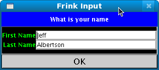
Making Interactive Interfaces
The following program demonstrates an idiom for creating a simple
interactive GUI that finds roots of numbers until you cancel. The while
loop exits when the user cancels calculations. Previous
results are displayed to the user at the top of the input dialog, and the
user's previous input is maintained (verbatim) in the input fields.
n = "10000"

    r = "2"

    message = "Find roots of a number"

    while [n, r] = results = input[message, [["Number", n], ["Root", r]]]

    {

       [num, root] = eval[results]  // Turn into numbers

       val = num^(1/root)

       message = "$n^(1/$r) = $val"

       println[message]

    }
This code works whether the user is running with a Swing or AWT or Android GUI, or in text mode. The user cancels input by closing the input dialog (in Swing or AWT), hitting the "back" button on Android, or with end-of-file (EOF) in text mode (EOF can be simulated by Control-D on Unixlike systems, Control-Z on Windows.)
Note that the idiomatic use of the "eval" function to turn the string
inputs into Frink expressions. This means that the user can enter any
expression that Frink understands, such as " 2+2
", " 1
trillion
", " sin[30 degrees]
" or " 32
m^2
". It's like a generalized calculator inside of a specialized
calculator!
Output
To print, use the print
or println
functions,
each of which take one argument. The only difference is that println
sends a linefeed afterwards.
println["The volume of the sphere is " + (volume ->
    ft^3) + " cubic feet."]
Boolean Operators
I'm just going to list a forest of cryptic boolean expressions here without
explanation. You pick out the ones you like. They all work, and there are
usually multiple equivalents for the same thing, taken from different
languages. I've tried to keep precedence the same as Java. There is no
difference between the different versions of, say, and
, AND
,
and &&
.
true TRUE false FALSE == != <> < <= > >= && and
    AND || or OR ! NOT not nand NAND nor NOR xor XOR implies IMPLIES
Three-Way Comparison
The three-way comparison operator, <=>
, also called the
"spaceship" operator, compares two arguments and returns their relative
ordering:
For a <=> b
, this returns:
-
-1ifa < b -
0ifa == b -
1ifa > b
These are the values expected by ordering functions, such as those used in user-defined.
Dictionaries
A dictionary is an associative data structure that lets you map arbitrary
keys to values (currently, keys can be strings, units, (that is, numbers),
sets, other dictionaries, arrays, date/time values, or objects created from
a class
.)
The syntax is identical to the syntax for array element manipulation. (This means that you can switch back and forth between an array and (sparse) dictionary representation for integer-indexed data structures!)
Create an empty dictionary using new dict
a = new dict
// Construct a dictionary
    a@"one" = 1

    a@"two" = 2

    a@"three" = 3
a@"one"
b = new dict
// Construct a dictionary
    b@1 = "one"

    b@2 = "two"

    b@3 = "three"
b@1
one
You can also enumerate over [key, value]
pairs directly in a
dictionary. They are not returned in any guaranteed order.
for [key, value] = a

       println["$key = $value"]
    two = 2

    one = 1

    three = 3
Dictionary Constructors
Create an empty dictionary:
a = new dict
Create a dictionary from an array (or enumerating expression) where each element in the array is a two-item list which are treated as a key and a value:
array = [["one", 1], ["two", 2]]  // A literal array

    d = new dict[array] // Create a dict from the array

    d@"one"  // Look up an item
1
You can also turn an array (or other types) into a dictionary by calling
the toDict[array]
function on it, which behaves exactly
like calling the single-argument constructor above.
Create a dictionary from two arrays (or enumerating expressions) where the first array contains keys and the second array contains values. The first element in the keys array will be matched with the first element in the values array.
keys = ["one", "two"]

    values = [1,2]

    d = new dict[keys, values]

    d@"one"// Look up an item
1
d
// print the dictionary[[one, 1], [two, 2]]
Dictionary Methods
You can get an enumeration of the keys in a dictionary by using the keys
function. This function does not return the keys in any
defined order, but you can sort them with thesorting
functionsbelow.
for key = keys[a]

       println[ "$key = " + a@key]
    two = 2

    one = 1

    three = 3
A dictionary can be queried to see if it contains a specific key using the containsKey[key]
method:
b.containsKey[1]
true
b.containsKey[4]
false
Entries in a dictionary can be removed with the remove[key]
method. This returns the value
corresponding to the key, or the special value undef
if that
key is not in the dictionary.
b.remove[1]
one
b.remove[4]
undef
You can invert the contents of a dictionary by using the invert
method which returns a new dictionary with key-value
pairs reversed. If the values are not hashable, this will print a
warning. If the same value appears multiple times, this will print a
warning.
c = b.invert[]
[[one, 1], [two, 2], [three, 3]]
A dictionary can be cleared by using the clear
method:
    a.clear[]

    a
[]
A dictionary is often used to count occurrences of an item.
The increment[key, increment]
method increments
the value corresponding to the specified key by the specified count. It
returns the new total.
    d=new dict

    d.increment["a", 1]

    d.increment["a", 1]

    d.increment["b", 1]

    d
    [[a,2],

     [b,1]]
A dictionary is often used to store a list of occurrences corresponding to
the specified key. The
functions addToList[key, value]
or addToSet[key, value]
pushes the specified
value onto the list or set corresponding to the key and returns the new
list or set.
    d=new dict

    d.addToList["a", 1]

    d.addToList["a", 2]

    d.addToList["b", 3]

    d
    [[a, [1, 2]],

     [b, [3]]]
    d=new dict

    d.addToSet["a", 1]

    d.addToSet["a", 2]

    d.addToSet["b", 3]

    d
    [[a, [1, 2]],

     [b, [3]]]
Sets
A set is a data structure that contains items with no duplicates. A set
can currently contain strings, units, (that is, numbers),
other sets, dictionaries, or objects created from a class
.)
You simply create an empty set using new set
, a literal set by
calling something like new set[1,2,3]
, or turn an array or
enumerating expression into a set by calling toSet[expr]
.
a = new set
// Construct a set
b = new set[1,2,3]
// Construct a set with
    the specified elements
c = [3,6,9]  // Create an array

      d = toSet[c] // Create a set from the
       array
Note that sets do not preserve any order of the items contained in them. There are a variety of methods for modifying sets:
Items are inserted into a set using the put
method:
    a.put[1]

    a.put[2]
[1,2]
Multiple items from an array, set, or other enumerating expression can be
inserted into a set as separate items using the putAll
method:
    b = new set

    c = [1,2,3]

    b.putAll[c]
[2,3,1]
Items are removed from a set using the remove
method:
    a.remove[2]

    a
[1]
A set can be tested to see if it contains a value by using the contains
method:
a.contains[1]
true
You can get a shallow copy of a set by calling its .shallowCopy[]
method.
    b = a.shallowCopy[]

    b.put[2]

    b
[1,2]
A set can be cleared by using the clear
method:
    a.clear[]

    a
[]
You can also enumerate over values contained in a set:
for value = a

       println[value]
The following demonstrates turning an enumerating expression into a set (the lines[url]
function returns an enumerating expression
of all of the lines in a file,) turning that into an set (to remove
duplicates) and sorting it (implicitly turning it into an array in the
process.) The result is a sorted array containing all of the unique lines
in a file, discarding duplicates.
sort[toSet[lines["file:myfile.txt"]]]
To obtain all of the possible subsets of the elements in the set, you
can use the set.subsets[]
method. This returns an
enumerating expression which iterates through allt he subsets of items in
the set, including the empty set and the original set itself. Each
return value is itself an set of elements.
    a = new set[1,2,3]

    println[a.subsets[]]
[[], [1], [2], [1, 2], [3], [1, 3], [2, 3], [1, 2, 3]]
You can also request the subsets of the set and exclude either the empty
set or the original set by using the set.subsets[allowEmptySet, allowOriginalSet]
method. If allowEmptySet
is true
, the empty set
will be returned as one of the elements. If false
, the empty
set will be excluded. If allowOriginalSet
is true
, the full original set will be returned as one of the
elements. If false
, the full original set will be excluded,
and only "proper" subsets will be returned.
    a = [1,2,3]

    println[a.subsets[false, false]]
[[1], [2], [1, 2], [3], [1, 3], [2, 3]]
Note that output of the empty set and the original set are suppressed in the example above.
Set Functions
The following functions operate on sets:
Function Description union[ a , b ] Returns a new set whose value is the union of setsa
and b
. (Sometimes written a ∪ b
.) In other words, the new set contains all of the elements that exist in either
set a
or
set b
.
intersection[ a
, b
]
Returns a new set whose value is the intersection of sets a
and b
. (Sometimes written a ∩ b
.) In other words, the new set contains only the elements that exist in both
set a
and
set b
.
setsIntersect[ a
, b
]
Returns true if the two sets have a non-empty intersection. That is, both sets contain at least one element in common.
setDifference[ a
, b
]
Returns a new set whose value is the difference of sets a
and b
. (Sometimes written a - b
.) In other words, the new set contains only the elements that exist in set a
but not
in set b
. If the arguments are not sets, this tries to coerce the arguments into sets, so it can be used to get the differences of arrays as sets, for instance. Note that ordering will be lost when differencing arrays.
isSubset[ a
, b
]
Returns true if sets a
is a subset of set b
. (Sometimes written a ⊆ b
.) In other words, this returns true if all of the elements in set a
are also contained in set b
. Note that this does not test that this is a "proper" subset.
See below.
isProperSubset[ a
, b
]
Returns true if sets a
is a proper
subset of set b
. (Sometimes written a ⊂ b
.) In other words, this returns true if all of the elements in set a
are also contained in set b
and
set a
also has fewer members than b.
toSet[ x
]
Turns the specified expression into a set, if possible. This works with enumerating expressions, arrays, or simple expressions (making a single-item set out of the latter.)
length[ a
]
Returns the cardinality of the set, that is, the number of items it contains.
Common Functions
The most common trigonometric functions are built in. They, as everything else in Frink, are best used when you explicitly specify the units. For the following functions, input should be an angle, and output will come out dimensionless. (If no unit is specified for input, it should act like radians, because radians are dimensionless units and really indistinguishable from pure numbers.)
sin[90 degrees]
cos[2 pi radians]
tan[30 arcsec]
sec[45 degrees]
csc[pi/2 radians]
cot[30 arcsec]
sinh[90 degrees]
cosh[2 pi radians]
sech[2 pi radians]
tanh[30 arcsec]
For inverse operations, the input must be dimensionless, and the output will come out in angular units. (Radians, by default.) This is easily converted to whatever angular units you want, as above. You don't see that the output is in radians because radians are essentially dimensionless numbers. You just gotta be a bit careful with angles.
arcsin[.1] -> degrees
arccos[1/2] -> radians
arcsin[.1] -> degrees
arccsc[3/2] -> radians
arcsec[3/2] -> radians
arccot[1/2] -> radians
arctan[3 inches/(1 foot)] -> arcminutes
(Returns a value in the range [-π/2, π/2])
arctan[3 inches, 1 foot] -> degrees
(Calculates arctan[x/y]
corrected for the proper quadrant.
Returns a value in the range [-π, π])
Formatting Functions
The following functions can be used to format numeric and unit expressions to a variety of formats.
Note:
the ->
operator is a formatting operator
that always returns a string
, so you can't format it any
further.
This is wrong:
a = 10 USD -> Euro   // Creates a string (don't do this!)

    format[a, "Euro", 2] // format won't work on a string!
This is right, and only converts and formats on output, which is usually what you want to do:
    a = 10 USD

    format[a, "Euro", 2]
formatFix[num, divideBy, decPlaces]
formatFixed[num, divideBy, decPlaces] Fixed-decimal-places format: Divides
num
by divideBy
and returns a string with a fixed number ( decPlaces
) of digits after
the decimal point. (If the number is dimensionless without size, divideBy
should be 1
). For example:
format[3 meters, feet, 2]
9.84
If divideBy
is a string, this evaluates the string,
expecting a unit to be returned, and both divides by this unit and
concatenates the string after the result:
format[3 meters, "feet", 2]
9.84 feet
Note: This function is somewhat deprecated for several reasons:
- It requires additional work behind the scenes which makes it slower. (That is, it needs to predict how many digits will be in the result after division, and then has to increase its working precision to calculate the full number of digits after the decimal point.)
- It is not a very readable representation for very large or very small numbers.
- It loses information for small numbers (less-significant digits may be lost or rounded or the number may be lost entirely.)
- It is rarely a good choice for large numbers, as many of the decimal places will be meaningless or displayed as zero.
- It's not quite as flexible as the other functions. It will not work if its arguments are not real numbers ( e.g. complex numbers or intervals. The other formatting functions will work in this case.)
The previous behavior of the format
function was preserved
to keep old programs working, but the default behavior of format
may
change in the future to another one of
the formatting functions below. The formatFix
and formatFixed
functions (which are identical to each other)
will keep their current behavior, so it's probably better to use formatFix
instead of format
to future-proof
your programs if this is the behavior your want to keep.
num
by divideBy
and returns a string in scientific notation with decPlaces
decimal digits. (If the number is dimensionless without size, divideBy
should be 1
). For example: formatSci[1 mm, feet, 2]
3.33e-3
If divideBy
is a string, this evaluates the string,
expecting a unit to be returned, and both divides by this unit and
concatenates the string after the result:
formatSci[1 mm, "feet", 4]
3.281e-3 feet
formatSig[num, divideBy, decPlaces]
Significant Figures format:
Divides num
by divideBy
and returns a string with decPlaces
significant digits. This may be a normal number or a number in scientific format, depending on the size of the number. (If the number is dimensionless without size, divideBy
should be 1
). For example: formatSig[100 mm, feet, 2]
0.34
If divideBy
is a string, this evaluates the string,
expecting a unit to be returned, and both divides by this unit and
concatenates the string after the result:
formatSig[100 mm, "feet", 3]
0.328 feet
formatEng[num, divideBy, decPlaces]
Engineering format:
Divides num
by divideBy
and returns a string in "engineering" format (that is, in scientific mode or normal mode where exponents are a multiple of 3,) so that they can be easily read as milli-, kilo-, mega-, etc. with decPlaces
significant digits. (If the number is dimensionless without size, divideBy
should be 1
). For example: formatEng[1000 miles, m, 4]
16.09 e+6
If divideBy
is a string, this evaluates the string,
expecting a unit to be returned, and both divides by this unit and
concatenates the string after the result:
formatEng[29000 feet, "meters", 3]
8.84e+3 meters
The following compares the output of the various formatting functions by
displaying -2/3 * 10^n
for various integer values of n
.
formatSig
formatSci
formatEng
format
, formatFix
-6.66667e-12
-6.66667e-12
-6.66667e-12
0.000000
-6.66667e-11
-6.66667e-11
-66.6667e-12
0.000000
-6.66667e-10
-6.66667e-10
-666.667e-12
0.000000
-6.66667e-9
-6.66667e-9
-6.66667e-9
0.000000
-6.66667e-8
-6.66667e-8
-66.6667e-9
0.000000
-6.66667e-7
-6.66667e-7
-666.667e-9
-0.000001
-6.66667e-6
-6.66667e-6
-6.66667e-6
-0.000007
-6.66667e-5
-6.66667e-5
-66.6667e-6
-0.000067
-6.66667e-4
-6.66667e-4
-666.667e-6
-0.000667
-6.66667e-3
-6.66667e-3
-6.66667e-3
-0.006667
-6.66667e-2
-6.66667e-2
-66.6667e-3
-0.066667
-0.666667
-6.66667e-1
-666.667e-3
-0.666667
-6.66667
-6.66667
-6.66667
-6.666667
-66.6667
-6.66667e+1
-66.6667
-66.666667
-666.667
-6.66667e+2
-666.667
-666.666667
-6666.67
-6.66667e+3
-6.66667e+3
-6666.666667
-66666.7
-6.66667e+4
-66.6667e+3
-66666.666667
-666667
-6.66667e+5
-666.667e+3
-666666.666667
-6.66667e+6
-6.66667e+6
-6.66667e+6
-6666666.666667
-6.66667e+7
-6.66667e+7
-66.6667e+6
-66666666.666667
-6.66667e+8
-6.66667e+8
-666.667e+6
-666666666.666667
-6.66667e+9
-6.66667e+9
-6.66667e+9
-6666666666.666667
-6.66667e+10
-6.66667e+10
-66.6667e+9
-66666666666.666667
-6.66667e+11
-6.66667e+11
-666.667e+9
-666666666666.666667
-6.66667e+12
-6.66667e+12
-6.66667e+12
-6666666666666.666667
Rounding Functions
Function Definition floor[x] Returns largest integer <= x floor[x,y] Rounds x down to the nearest multiple of y. For example,floor[3.14159, 0.001]
returns 3.141
This can be used with units of measure, for example: floor[23 hours, day]
returns a unit equal to 0 days
.
ceil[x]
Returns smallest integer >= x
ceil[x,y]
Rounds x up to the nearest multiple of y. For example, ceil[3.14159, 0.01]
returns 3.15
. This can be used with units of measure, for example: ceil[13 hours, day]
returns a unit equal to 1 day
.
round[x]
Rounds to nearest integer
round[x, y]
Rounds x
to nearest multiple of y
. This can be used with units of measure, for example: round[13 hours, day]
returns a unit equal to 1 day
.
int[x]
Truncates decimal places to produce integer
trunc[x]
Truncates decimal places to produce integer
numerator[x]
Returns the numerator of a rational, dimensionless number. If the number is not rational and dimensionless, simply returns the number.
denominator[x]
Returns the denominator of a rational number. If the number is not rational and dimensionless, simply returns 1.
Number Theory
Some functions for number theory and factorization are available.
Note: If you're doing number-theoretical work with very large integers, please see thesection of the documentation for ways to greatly improve integer performance.
Function Description bitLength[ x ] Returns the number of bits in the minimal two's-complement representation of an integer, excluding a sign bit. In other words, this returns the index of the highest bit that differs from the sign bit. getBit[ num , bit ] Returns an integer, either 0 or 1, indicating the value of the specified bit in an integer. Bit 0 is the least-significant bit. The number is treated as a two's-complement representation with infinite length. That is, the high bits on a negative number will always be 1, and the high bits on a positive number or zero will always be 0. getLowestSetBit[ num ] Returns the index of the rightmost (lowest-order) one bit in an integer (the number of zero bits to the right of the rightmost one bit). Returns -1 if the integer contains no one bits. shiftLeft[ num , bits ] Shifts the bits of an integer left by the specified number of bits. New bits will contain zero. This is equivalent to multiplying by 2 bits but is usually more efficient. shiftRight[ num , bits ] Shifts the bits of an integer right by the specified number of bits, losing the bits pushed off the right side. This is equivalent to performing adiv
by 2 bits
but is usually more efficient.
bitAnd[ n
, m
]
Returns the bitwise AND
of two integers, treated as two's complement numbers with infinite sign bits.
bitOr[ n
, m
]
Returns the bitwise OR
of two integers, treated as two's complement numbers with infinite sign bits.
bitXor[ n
, m
]
Returns the bitwise XOR
(exclusive-or) of two integers, treated as two's complement numbers with infinite sign bits.
bitNot[ n
]
Returns the bitwise NOT
of an integer, treated as a two's complement number with infinite sign bits. This means that performing a bitNot
on a positive number will return a negative number, and vice-versa. This may be unexpected if you're unfamiliar with two's complement notation, but functions like getBit[num, bit]
and bitLength[num]
will do the right thing, and will handle all leading sign bits correctly without you needing to specify the length of your numbers. Please look up two's complement number representation if you're unfamiliar with this.
bitNand[ n
, m
]
Returns the bitwise NAND
(an AND followed by a NOT) of two integers, treated as two's complement numbers with infinite sign bits. See notes about bitNot[num]
above.
bitNor[ n
, m
]
Returns the bitwise NOR
(an OR followed by a NOT) of two integers, treated as two's complement numbers with infinite sign bits. See notes about bitNot[num]
above.
gcd[ x
, y
]
Returns the greatest common divisor of the integers x
and y
.
lcm[ x
, y
]
Returns the least common multiple of the integers x
and y
.
isPrime[ x
]
Returns false if the integer x
is composite, true if the number is prime (or probably prime.) This test uses trial division and then Rabin-Miller strong pseudoprime tests to determine primality. The bases used in the Rabin-Miller test are known to prove
primality for numbers smaller than 3,317,044,064,679,887,385,961,981, (see Sorenson and Webster
) but for larger numbers this function can erroneously declare a composite number to be prime. (If it returns false, the number is definitely composite.)
If the number is larger than this, the test is performed against 78
random prime bases. This gives a very
small probability of
about 1 in 10 47
that the function may return true
for a composite number. (And that's a worst-case;
for randomly-chosen large numbers, the probability of error is actually
far, far lower for most numbers, especially big ones. The above
assumes the ridiculously low estimate that the pseudoprime test fails
1/4 of the time. The reality is orders of magnitude lower. For better
estimates, see Probable primes: How Probable?
and remember to
raise each number given in that table to the 78th power!
)
It is more likely that any of the following will happen:
- Your hardware will fail and return the wrong answer (perhaps due to a cosmic ray hitting it.)
- You'll flip a coin 156 times in a row and it will land on "heads" every time.
- You'll play roulette and your number will get picked 29 times in a row.
- You'll test a trillion numbers every second for the known lifetime of the universe and you'll still only have a miniscule 1 in 10 17 chance of getting a single wrong answer.
And these are ridiculously generous estimates. The actual probability of failure is usually astronomically lower than this.
As of the 2005-11-13 release, isPrime[x]
was
extended to automatically use a faster Lucas-Lehmer test if x
is
of the form 2 n
-1 ( i.e.
Mersenne numbers). Note that
the Lucas-Lehmer test is sufficient to prove
primality for
numbers of this form, regardless of their size.
Also note that isPrime[1]
will return true
.
This simplifies recursive factor-finding algorithms, but I know it may
not match the modern definition of primes. This behavior may change,
so try not to rely on it.
Frink is not vulnerable to the attacks in the very interesting Prime and Prejudice paper. You can test it with the PrimeAndPrejudice.frink sample program.
factor[ x ] Returns the prime factors of an integerx
as a two-dimensional list. This uses trial division, then the Pollard p-1
method, and then the Pollard Rho method to find factors. The factor list consists of a list of pairs of prime factors and the exponent of each factor:
factor[1000]
[[2, 3], [5, 3]]
This indicates that the prime factors of 1000 are 2 3 * 5 3 .
factorFlat[ x ] Returns the prime factors of an integerx
as a one-dimensional list. This uses trial division, then the Pollard p-1
method, and then the Pollard Rho method to find factors. The factor list consists of a list of prime factors, each possibly repeated. This performs identically to the factor[x]
function above; the output format is just different.
factorFlat[1000]
[2, 2, 2, 5, 5, 5]
n
, not just prime factors
. The optional arguments include1
and includeN
indicate if the numbers 1 and n are to be included in the results. If the optional argument sort
is true, the results will be sorted. If the optional argument onlyToSqrt
=true, then only the factors less than or equal to the square root of the number will be produced. It currently returns an array, but that may change to an enumerating expression someday to be more memory-efficient for numbers with huge amounts of factors.
JacobiSymbol[ a,n
]
Returns the Jacobi symbol (often written as (a/n) ) of the integers a
and n
. n
must be a positive, odd integer. This function is used in factorization and primality testing. The Jacobi symbol is a generalization of the Legendre symbol, so it can be used to calculate the Legendre symbol of two numbers. (The Legendre symbol is only defined if n
is prime.)
isStrongPseudoprime[ num
, base(s)
]
Returns true if num
is a strong pseudoprime to base base
. If this returns false, the number is definitely composite. If it returns true, the number may
be prime. This does not
prove that a number is actually prime, as numbers can fail this test for up to 1/4 of bases. This can be used as a component of a prime sieving algorithm (but be sure to do things like verify that the number is odd first!)
The argument base
can also be an array of integers, in
which case all of the bases are tested, bailing out when the number is
known to be composite. This may be slightly faster (and easier to
code) in some cases. You may be able to use this along
with minimal sets of bases
(link opens in new window) to
make an even faster primality test.
While the above paragraph correctly states that this test can fail for up to 1/4 of bases, the actual failure rate for larger numbers is many orders of magnitude smaller than that! See Probable primes: How Probable? (link opens in new window) for an estimate of how much lower the failure rate becomes.
nextPrime[n]
Returns the next prime number greater than
n
. The value of n
may be any real number. This method uses a wheel factoring method to completely avoid testing composite numbers with small factors.
previousPrime[n]
Returns the previous prime number smaller than
n
. The value of n
may be any real number. If n
n is smaller than 2, this returns undef
. This method uses a wheel factoring method to completely avoid testing composite numbers with small factors.
primes[]
Returns an infinite enumerating expression that lists all of the prime numbers in ascending order. Note that this will produce infinite output if you even try to print it, so you probably want to call it from a for
loop or from something like first[primes[], 100]
partitionCount[n]
Returns the number of ways that the integer n can be partitioned. This uses Euler's pentagonal number algorithm to find the partition count somewhat efficiently, and caches the results so subsequent calls to this function will be efficient.
partitions[n]
Returns an enumeration of the partitions of the integer n. For example:
        for a = partitions[4]

           println[a]
        [4]

        [3, 1]

        [2, 2]

        [2, 1, 1]

        [1, 1, 1, 1]
partitionsCompact[n, countPermutations=false]
Like the partitions
function above, but returns a more compact enumeration of the partitions of the integer n. Each list contains [num, count] pairs indicating the number and its count in a partition. For example, compare the following representation with the one from the partitions
function above.
        for a = partitionsCompact[4]

           println[a]
        [[4, 1]]

        [[3, 1], [1, 1]]

        [[2, 2]]

        [[2, 1], [1, 2]]

        [[1, 4]]
If the optional argument countPermutation
is true
, then each element also contains the number of
possible permutations of the list.
binomial[m,n]
Returns the binomial coefficient. This is of the number of ways m
things can be chosen n
at a time, with order being unimportant. This is sometimes called "m choose n" or "m C n". This is equivalent to m!/(n!*(m-n)!) although calculating that way often leads to way-too-big numbers. For example, binomial[10000, 9998]
is equal to 49995000, but if you calculated it naively, you'd have to calculate 10000! which is a 35660-digit number, and divide it by another huge number, which could be inefficient and slow.
eulerPhi[n]
Returns Euler's Totient (also known as the phi function or Euler's Phi) of the given integer. This is the number of positive integers less than n that share no factors with n.
factorial[n]
Returns the factorial of the specified non-negative integer. This is the same as the factorial operator !
.
Reminder:
the factorial
of a non-negative integer n
is the product of all the
numbers from 1 to n
. For example, the factorial 6!
is equal to 1 * 2 * 3 * 4 * 5 * 6
, or 720
factorialRatio[m, n]
Efficiently calculates the ratio of two factorials m! / n!
, using a binary
splitting algorithm
. This is used internally in functions like binomial[m, n]
. Using this function is much
faster than calculating the result naïvely.
Other number-theoretical functions, such as those for calculating the values of theRiemann Zeta function may be available in theSample Programs library.
Other Functions
Function Definition array[x]toArray[x] Turns the specified expression into an array. This works with enumerating expressions, sets, dictionaries, objects created from a
class
, or simple expressions (making a single-item array out of the latter.)
flatten[array]
Flattens a possibly multi-dimensional array into a 1-dimensional array. For example, flattening the array [1,[2,[3,4]],5]
results in [1,2,3,4,5]
.
toString[x]
Turns the specified expression into a string. The string representation is exactly the same as it would be from printing the expression orinterpolating it into a string.
deepCopy[x]
Perform a recursive deep copy of all the parts of a container class. The function can be called with any expression type. The function currently deep copies everything contained in arrays, dictionaries, sets, OrderedLists, RingBuffers, and objects created from a class
specification, and everything contained within them. It is thus useful for copying nested data structures, multi-dimensional arrays (which are arrays of arrays, etc.) and prevents modification of the original or the copy from changing the other. It does not
currently deep copy Java objects, nor Java arrays.
inv[x]
Reciprocal 1/x
recip[x]
Reciprocal 1/x
sqrt[x]
Square root
log[x]
Common logarithm, base 10. This returns exact integers or rational numbers in cases when arguments are integers and results are integers or 1 divided by an integer.
ln[x]
Natural logarithm, base e
log[x, b]
Logarithm of the number x
to the base b
, which could also be written ln[x] / ln[b]
(which works for any base as long as the logarithms are taken to the same base) but this version returns exact integers or exact rational numbers when arguments are integers when the result is an integer or 1 divided by an integer.
exp[x]
e x
Re[x]
The real part of x. Note that the result will have the same dimensions as the argument.
Im[x]
The imaginary part of x as a real number. Note that the result will have the same dimensions as the argument.
conjugate[x]
Returns the complex conjugate of the specified number. Note that the result will have the same dimensions as the argument.
sinh[x]
Hyperbolic sine of x, or (e x
- e -x
)/2
csch[x]
Hyperbolic cosecant of x, or 1/sinh[x], or 2/(e x
- e -x
)
cosh[x]
Hyperbolic cosine of x, or 1/sech[x], or (e x
+ e -x
)/2
sech[x]
Hyperbolic secant of x, or 1/cosh[x], or 2/(e x
+ e -x
)
tanh[x]
Hyperbolic tangent of x, or sinh[x]/cosh[x]
coth[x]
Hyperbolic cotangent of x, or (e 2z
+ 1) / (e 2z
- 1)
arcsinh[x], asinh[x]
Inverse hyperbolic sine of x, or ln[x + sqrt[1 + x^2]]
arccosh[x], acosh[x]
Inverse hyperbolic cosine of x, or ln[x + sqrt[x-1] sqrt[x+1]]
arcsech[x], asech[x]
Inverse hyperbolic secant of x, or ln[sqrt[1/x - 1]*sqrt[1 + 1/x] + 1/x]
arccsch[x], acsch[x]
Inverse hyperbolic cosecant of x, or ln[sqrt[1 + 1/x^2] + 1/x]
arctanh[x], atanh[x]
Inverse hyperbolic tangent of x, or 1/2 (ln[1+x] - ln[1-x])
arccoth[x], acoth[x]
Inverse hyperbolic cotangent of x, or 1/2 ( ln[1 + 1/x] - ln[1 - 1/x] )
abs[x]
Absolute value. For complex arguments, returns complex number abs[x + iy] = sqrt[x^2 + y^2]
. For interval arguments, returns an interval (which may contain zero if the interval contains zero.) Note that the result will also have the same dimensions as the argument!
signum[x]
Returns the sign of the argument. For real-valued arguments, this returns (-1 if x<0), (0 if x==0), (1 if x>0). For complex arguments, returns x/abs[x]
. For intervals, returns an interval containing the signum of each endpoint (which may be collapsed to a single value if both endpoints have the same sign.) Note that the result will also have the same dimensions as the argument!
realSignum[x]
This is a more limited function that returns the sign of a real number, ignoring units of measure if they are present. For real-valued arguments, this returns (-1 if x<0), (0 if x==0), (1 if x>0). For all other arguments, this returns undef
.
random[x]
Pick a random integer between 0 (inclusive) and x
(exclusive.) If x
is an array, this returns a random item from the array.
random[min, max]
Pick a random integer between min (inclusive) and max (inclusive.) Note: To pick items from a discrete probability distribution, see the DiscreteDistribution.frink sample program.
randomFloat[ lower , upper ] Pick a uniformly-distributed random floating-point value in the specifed range. randomGaussian[ mean , sd ] Pick a normally-distributed (i.e. "bell curve") random floating-point value with the specified mean and standard deviation. randomBits[ numBits ] Generate a random positive integer containing numBits evenly-distributed binary bits. randomBytes[ numBytes ] Generate an array of random bytes containing numBytes elements as a Java array of byte. randomSeed[ seed ] To obtain repeatable results with a program that generates random numbers, sometimes it is desirable to use the same random sequence. This function seeds the random number generator with a known value. The seed must a number from -2 63 to 2 63 -1 (both inclusive.) bitLength[ int ] Returns the number of bits in the minimal two's-complement representation of an integer, excluding a sign bit. modPow[ base , exponent , modulus ] Perform the integer modular exponentiation ( base exponent mod modulus ) in an efficient manner. modDiv[ n , m , modulus ] Performs the integer modular division n/m mod modulus and returns the integer result if one exists, otherwise returnsundef
.
modInverse[ n
, modulus
]
Finds the integer modular inverse of n
to the base modulus
and returns the integer result if it is invertible, otherwise returns undef
. In other words, modInverse[n,m]
returns an integer x
such that (x * n) mod m == 1
.
min[ arg1
, arg2
]
Returns the smaller of the two arguments, or the first argument if they're equal.
min[ array
]
Returns the smallest item in the array.
max[ arg1
, arg2
]
Returns the larger of the two arguments, or the first argument if they're equal.
max[ array
]
Returns the largest item in the array.
clamp[ num
, min
, max
]
Returns the specified number, but limiting its value to lie between the specified minimum and maximum. This also works correctly when num
is an interval.
intersection[ arg1
, arg2
]
Returns the intersection of two intervals, or an interval and a real number. (Or two real numbers, but that rarely makes sense.) The return type in this case will be an interval or an ordinary real number. If there is no intersection between the arguments, the function will currently return undef
although this behavior may change to return an empty interval in the future. This function also works with dates and date intervals.
union[ arg1
, arg2
]
Returns the union of two intervals, or an interval and a real number. (Or two real numbers, in which case an interval containing both real numbers is returned.) The return type will be an interval or an ordinary real number if the two numbers are the same real number. This function also works with dates and date intervals.
isInteger[ expr
]
Returns true if the argument is a dimensionless integer, false otherwise.
isRational[ expr
]
Returns true if the argument is a dimensionless rational number (and not
an integer,) false otherwise.
isReal[ expr
]
Returns true if the argument is a real number (with or without dimensions, and not an interval,) false otherwise.
isComplex[ expr
]
Returns true if the argument is a complex number (with or without dimensions,) false otherwise.
isInterval[ expr
]
Returns true if the argument is an interval (with or without dimensions,) false otherwise.
isNegative[ expr
]
Returns true if the argument is a dimensionless negative number, false otherwise.
isPositive[ expr
]
Returns true if the argument is a dimensionless positive number, false otherwise.
isUnit[ expr
]
Returns true if the number is a unit of any type, including dimensionless numbers.
isArray[ expr
]
Returns true if the expression is an array, false otherwise.
isDict[ expr
]
Returns true if the expression is a dictionary, false otherwise.
isSet[ expr
]
Returns true if the expression is a set, false otherwise.
isDate[ expr
]
Returns true if the expression is a date/time, false otherwise.
isString[ expr
]
Returns true if the expression is a string, false otherwise.
sum[x]
Returns the sum of the elements of x
, which can currently be an array or an enumerating expression. If x
is of any other type, this simply returns x
. If the list is empty, this returns undef
. (There is no universal identity element for addition when units of measure may be present.)
sum[x, emptyValue]
Returns the sum of the elements of x
, which can currently be an array or an enumerating expression. If x
is of any other type, this simply returns x
. If the list is empty, this returns emptyValue
.
product[x]
Returns the product of the elements of x
, which can currently be an array or an enumerating expression. If x
is of any other type, this simply returns x
. If the list is empty, returns 1.
product[x, emptyValue]
Returns the product of the elements of x
, which can currently be an array or an enumerating expression. If x
is of any other type, this simply returns x
. If the list is empty, returns emptyValue
.
sleep[ time
]
Sleeps for the specified amount of time. The argument time
must have units of time, such as 1 s
or 4.9 minutes
or 1/30 s
.
binaryToGray[ num
]
Converts the specified number into its corresponding value in binary reflected Gray code. Example usage: binaryToGray[0b1111] -> binary
grayToBinary[ num
]
Converts a number from its value in binary reflected Gray code to its equivalent numeric value.
browse[ url
]
Launches the specified URL in the browser (or however your computer is set up to launch URLs.) This requires that your Java Virtual Machine and your operating system are configured correctly.
integerDigits[ num
]
Returns an array of the digits of the non-negative integer num
in base 10.
integerDigits[ num
, base
]
Returns an array of the digits of the non-negative integer num
in the specified base.
getExponent[ unit
, baseUnit
]
Returns the exponent for the specified base unit. The base unit can be specified as a string indicating the name of a base unit (e.g. "m"
for meters), a unit of measure, e.g. ( m
), or a string indicating the name of a base dimension (e.g. "length"
or "mass"
or "time"
. See thedefault
base dimension names. )
For example, to get the exponent corresponding to length (default unit is meters) all of the following are equivalent:
        getExponent[3 m/s^2, "length"]

        getExponent[3 m/s^2, "m"]

        getExponent[3 m/s^2, "meters"]

        getExponent[3 m/s^2, "feet"]

        getExponent[3 m/s^2, m]

        getExponent[3 m/s^2, 123.4 m]

        getExponent[3 m/s^2, 3 feet]
All of the above return the integer 1
, which is the
exponent for
length in the provided expression. Asking for "time"
or "s"
or s
would return -2
, the
exponent for the time dimension. Also note that exponents may be
rational numbers or zero.
Warning: You will very likely never need this function. If you're using it, you may be doing something sketchy and unwise and physically unrealistic, or attempting to subvert unit-checking, or missing better input/output routines. Stop and reconsider your life choices.
Fourier Transforms
Frink can perform Fourier transforms on 1- or 2- dimensional arrays, or on
images (by calling their toComplexArray[]
method. See theFourierImage.frink sample progam for a demonstration.) The functions are:
DFT[array, divFactor=-1, direction=1]
inverseDFT[array, divFactor=-1,
     direction=1]
Performs a Discrete Fourier Transform of the given array. The array may be 1- or 2-dimensional.
Since different fields of mathematics and engineering use different conventions for the Fourier transform, these functions allow you to (optionally) specify the scaling factor and sign convention.
The (optional) second argument divFactor sets the scaling factor for the results:
DFT inverseDFT divFactor = -1 (default) 1/n 1 divFactor = 0 1/sqrt[n] 1/sqrt[n] divFactor = 1 1 1/nThe (optional) third argument direction sets the sign used in the exponent.
DFT inverseDFT direction = 1 (default) e2 pi i j k / n
e-2 pi i j k / n
direction = -1 e-2 pi i j k / n
e2 pi i j k / n
The inverseDFT
function produces the inverse of the DFT
given by the DFT function. In fact, it just calls the DFT function
with appropriately-reversed parameters.
If you specified the optional second or third arguments for the DFT
function, you will need to pass in the same
arguments to the inverseDFT
function to get the inverse operation. This
function takes care of reversing them appropriately.
FFT[array, divFactor=-1, direction=1]
inverseFFT[array, divFactor=-1,
      direction=1]
DFT
and inverseDFT
functions above.
While this function is much faster than DFT
, be warned
that this will pad the array with zeroes to the next largest
power of 2.
It will thus give a result that is different than
DFT, often with more terms.
FFT is O(n log n) while DFT is O(n 2 ).
Cryptographic Functions
The messageDigest[...]
functions can calculate a variety of
cryptographic hashes of various strings. The parameters for all are of the
form:
messageDigest[input,algorithm]
Each function can take as input either a string or an array of Java bytes.
The algorithm
parameter is a string containing one of any
hashing algorithms your Java platform supports, which probably includes: "MD2", "MD5", "SHA", "SHA-256", "SHA-384", "SHA-512"
. You
can see the cryptoProviders.frink
sample program to see how to dump all message digest types available on
your virtual machine.
Note:
As of the 2016-09-29 release, the behavior of the messageDigest
functions may have changed. Previously, to turn
the characters of a Unicode string into bytes, the function used your
platform's default character encoding. Now the functions always convert
the bytes to UTF-8 before creating the digest. (Your default was likely to
have been UTF-8 already.) Using the default encoding made programs
non-repeatable from one machine to another. If you want to force a certain
encoding of Unicode strings into bytes, use the
stringToBytes[string,
   encoding]
function before calling these functions.
The following calculates the MD5 hash of the string "abc"
and
returns it as a hexadecimal string:
messageDigest["abc", "MD5"]
900150983cd24fb0d6963f7d28e17f72
The messageDigestInt
function returns the value as an integer,
which can then be displayed in various bases, have its individual bits
tested, etc.
messageDigestInt["abc","MD5"] -> octal
2200025023017151117541532261767645070277562
The messageDigestBytes
function returns the value as an
array of Java bytes. Note:
Most of the underlying cryptography
routines in Java work with arrays of bytes, as these are safer than Strings
which are immutable after construction and are eventually
garbage-collected. Using arrays of bytes means that you can zero-out input
buffers as soon as you're done with them.
messageDigestBytes["abc", "SHA-1"]
All Your Base Conversions...
Integer values can be converted to and from other bases (from 2 to 36 inclusive) in several ways. The following functions can be used to convert to or from other arbitrary bases.
Function Description base[x, b] Returns a string representing the integerx
in base b
base2[x] ... base36[x]
Returns a string representing the integer x
in the specified base.
base64[x]
Converts between integer and base-64 encoded strings. If passed an integer, returns a string representing the integer as a base 64-encoded value. This uses standard base-64 indices in the order A-Za-z0-9+/. If passed a base-64 encoded string, this returns an integer with the corresponding value.
parseInt[ str
]
Parses a string, containing digits 0-9 only, to an integer in base 10. This should contain no spaces or other text.
parseInt[ str
, base
]
Parses a string, treating it as if it's a number in the specified base. The string should contain no spaces or other text. The base can from 2-36 (inclusive) or 64, in which case it will use standard base64 encoding.
The following named base conversion functions can also be used. In the cases where several names are commonly used, all options are listed. All functions return strings.
Base Function Name(s) 2 binary 3 ternary, trinary 4 quaternary 5 quinary 6 senary, sexenary 7 septenary 8 octal, oct, octonary 9 nonary 10 decimal, denary 11 undenary 12 duodecimal, duodenary 13 tridecimal 14 quattuordecimal 15 quindecimal 16 hexadecimal, sexadecimal, hex 17 septendecimal 18 octodecimal 19 nonadecimal 20 vigesimal
The conversions can be performed by calling the named function, or by using
the conversion operator ( ->
). The following are all
equivalent, and all convert the number specified by the variable number
to a string in base 8.
    base[number, 8]

    base8[number]

    number -> base8

    octal[number]

    number -> octal

    oct[number]

    number -> oct
Use whichever is most convenient for you. (Note: the function version will be slighly faster.)
As noted above in thesection, you may input numbers in a specified base by following the number with two backslashes and the specified base:
100001000101111111101101\\2
1000_0100_0101_1111_1110_1101\\2
845FED\\16
845fed\\16
845_fed\\16
0x845fed
0x845FED
0xFEED_FACE
0b100001000101111111101101
0b1000_0100_0101_1111_1110_1101
Custom Base Conversions
The above base conversions assume that the characters are taken from an
alphabet like the one for base 36: "0123456789abcdefghijklmnopqrstuvwxyz"
, which is common and
reasonable. For example, hexadecimal uses the first 16 characters of
this, "0123456789abcdef"
. However, it's not as clear when you
go beyond base 36 what characters should be used. You can declare a custom
"alphabet" of any size to be used in base conversions.
For example, Bitcoin addresses use a base-58 alphabet consisting of the characters:
"123456789ABCDEFGHJKLMNPQRSTUVWXYZabcdefghijkmnopqrstuvwxyz"
Note that this alphabet does not include 0
(zero), O
(uppercase o), I
(uppercase i), l
(lowercase L), as those are indistinguishable in some fonts.
To convert a number to a string using this alphabet, you can use the base[num, alphabet]
function where alphabet
is a string which contains the character for the
"zero" position first. The radix will be equal to the number of characters
in the alphabet string. (In the below example, base 58.) The following
turns a numeric value into a Bitcoin address string:
alphabet = "123456789ABCDEFGHJKLMNPQRSTUVWXYZabcdefghijkmnopqrstuvwxyz"

    number = 0x00010966776006953D5567439E5E39F86A0D273BEED61967F6

    base[number, alphabet]
6UwLL9Risc3QfPqBUvKofHmBQ7wMtjvM
(Note that this alphabet does not have a zero as the first character (it has a 1,) so if you need to pad it to a certain length, you need to pad with the first character in the alphabet.)
Conversely, you can parse an integer with a custom alphabet by using the parseInt[str, alphabet]
function, which takes
the same format for its alphabet string. The example below parses a
Bitcoin address.
alphabet = "123456789ABCDEFGHJKLMNPQRSTUVWXYZabcdefghijkmnopqrstuvwxyz"

    str = "6UwLL9Risc3QfPqBUvKofHmBQ7wMtjvM"

    parseInt[str, alphabet]
25420294593250030202636073700053352635053786165627414518
(Note that the number obtained above is the decimal equivalent of the Bitcoin address encoded above; it could instead be formatted in hexadecimal or other formats.)
The strings are allowed to contain any Unicode characters. If you attempt
to parse a string that contains characters outside your alphabet, the
special value undef
will be returned.
Custom Base Conversion Examples
This section demonstrates some custom base conversions.
Devanagari
Devanagari digits are used in Hindi and Sanskrit, and occur in the Unicode
standard from \u0966
(zero) through \u096f
(nine). To output a Devanagari integer:
alphabet = char[0x0966 to 0x096f]

    base[1234567890, alphabet]
१२३४५६७८९०
Conversely, a Devanagari integer can be parsed with:
alphabet = char[0x0966 to 0x096f]

    parseInt["१२३४५६७८९०", alphabet]
1234567890
Unicode Superscripts
The Unicode standard has a non-contiguous hodgepodge collection of numerals that represent superscript numerals, like 10¹². If you want to typeset a string of numbers as superscripts on a Unicode-aware system, you can do something like this:
supAlphabet = "\u2070\u00b9\u00b2\u00b3" + char[0x2074 to 0x2079]

    "10" + base[23, supAlphabet]
10²³
Or, conversely, to parse a stream of these superscript numerals as a single number:
supAlphabet = "\u2070\u00b9\u00b2\u00b3" + char[0x2074 to 0x2079]

    parseInt["²³", supAlphabet]
23
Complaint: : Note that almost all fonts make Unicode superscript numbers look different and not line up. Does your font look uniform here? Mine decidedly does not.
10¹²³⁴⁵⁶⁷⁸⁹⁰
Unicode Subscripts
Unicode numerical subscripts are more uniform and contiguous than
superscripts, thankfully. They occupy a contiguous range from \u2080
to \u2089
.
If you want to typeset a string of numbers as subscripts on a Unicode-aware system, you can do something like this:
    subAlphabet = char[0x2080 to 0x2089]

    "1000" + base[24, subAlphabet]
1000₂₄
If you want to parse a string of these subscripts as a single number, you can do something like this:
subAlphabet = char[0x2080 to 0x2089]

    parseInt["₄₂", subAlphabet]
42
Unicode Operators
Frink can parse Unicode characters that are commonly used as mathematical operators. This allows you to cut-and-paste some mathematical expressions without modification and handle them correctly.
Unicode superscript numerals can be used to perform exponentiation, such as 10⁻²³
, which is equivalent to 10^-23
, or x³
, which is equivalent to x^3
.
Note:
Web pages usually won't
use Unicode superscript
numerals, but rather <SUP>
tags for superscripts which
means that you probably won't be able to paste equations in directly.
The Unicode standard has a non-contiguous hodgepodge collection of numerals that represent superscript numerals. The only superscript characters currently recognized are the following:
Character Unicode Codepoint Description ⁰ \u2070 Superscript 0 ¹ \u00b9 Superscript 1 ² \u00b2 Superscript 2 ³ \u00b3 Superscript 3 ⁴ \u2074 Superscript 4 ⁵ \u2075 Superscript 5 ⁶ \u2076 Superscript 6 ⁷ \u2077 Superscript 7 ⁸ \u2078 Superscript 8 ⁹ \u2079 Superscript 9 ⁺ \u207a Superscript plus (must precede digits) ⁻ \u207b Superscript minus (must precede digits)
You can use the toUnicodeSuperscript[int]
function to
turn an integer into a string composed of Unicode superscript digits in
base 10.
You can use the toUnicodeSubscript[int]
function to
turn an integer into a string composed of Unicode subscript digits in
base 10.
In addition, some Unicode characters can be used as synonyms for other mathematical operators.
Character Unicode Codepoint Description × \u00d7 Unicode MULTIPLICATION SIGN, synonym for multiplication*
operator
⋅
\u22c5
Unicode DOT OPERATOR, synonym for multiplication *
operator. Unicode says "preferred to \u00b7 for denotation of multiplication"
·
\u00b7
Unicode MIDDLE DOT, synonym for multiplication *
operator
÷
\u00f7
Unicode DIVISION SIGN, synonym for division /
operator
As an example, the following is parsed correctly by Frink, as it uses Unicode (and not HTML) markup:
ρ = 6.02×10²³ amu ⋅ (6 m³)⁻¹
Note that Frink does not currently output Unicode, nor give you simplified ways to key in Unicode characters.
Strings
Text surrounded by double quotes is a string.
"My hovercraft is full of eels."
My hovercraft is full of eels.
If you need to put a literal double-quote inside a string, precede it with a backslash:
"If you believe in the hypothetical \"Z-Axis\""
If you believe in the hypothetical "Z-Axis"
Backslashes have a special meaning within double-quoted and triple-quoted strings. They may precede a special character, as follows:
String Description \\ Places a single backslash into the string. \t Places a tab character into the string. \n Places a newline character(s) into the string. The exact characters inserted follow your platforms's Java-defined settings for the newline character, which may be one character or two. \r Places a return character into the string. \" Places a double-quote character into the string. \u XXXX Places a Unicode character into the string, where XXXX is a 4-digit hex value for the Unicode codepoint. For more information, see thesection of the documentation. \u{ XXXXXX } Places a Unicode character into the string, where XXXXXX is a 1- to 6-digit hex value for the Unicode codepoint. For example, to create a string with a cat face, you would use"\u{1f638}"
(this is the Unicode character "GRINNING CAT FACE WITH SMILING EYES".) For more information, see thesection of the documentation.
A single backslash preceding any other character simply inserts the following character into the string (and removes the backslash.)
Strings can be concatenated using the +
operator. If either
side of a +
operator is a string, the values will be
converted to strings before concatenation.
Unicode in Strings
For internationalization, Frink allows Unicode characters anywhere. Strings can contain Unicode characters, indicated in one of a few ways:
-
Directly entered with a Unicode-aware editor. If you do
have a nifty editor that handles Unicode, or other character encodings, you can write your Frink program in full Unicode, and load it using the
--encoding strcommand-line switch. -
\ufollowed by exactly 4 hexadecimal digits [0-9a-fA-F] indicating the Unicode code-point. For example,"\u2764"indicates the Unicode character "HEAVY BLACK HEART". -
\u{XXXXXX}whereXXXXXXis anywhere from 1 to 6 hexadecimal digits. For example,"\u{1f435}"is the Unicode character "MONKEY FACE". Note that using this format is required because the hexadecimal value has more than 4 digits. -
High Unicode characters (those with value higher than
\uFFFF) can also be represented as a Unicode "surrogate pair." For example, the Unicode character "MONKEY FACE" can also be represented as two 4-hex-digit characters:"\ud83d\udc35". This is for compatibility with environments (such as Java) that represent a character as 16 bits. (TheinputForm[expr]function will produce this format for cross-platform and cross-Java-version compatibility.)
The latter two allow Unicode characters to be placed into any ASCII text file, and edited by programs that don't understand Unicode.
"The symbol for micro is \u00b5"
The symbol for micro is µ
Unicode Character Codes
You can convert a character to its Unicode character code by using the char[x]
function.
If passed an integer, it returns the character with that Unicode character code:
char[00b5\\16]
// Base 16, micro character as above.
µ
If passed a single-character string, it returns the Unicode character code:
char["A"]
65
If passed a multiple-character string, it returns the Unicode character code for each character in an array:
char["Frink"]
[70, 114, 105, 110, 107]
If you always need an array of character codes, use the chars[x]
function which turns a string into an array of
character codes, even when passed a string containing only one character.
chars["F"]
[70]
You can also obtain the results in a different base:
hex[chars["Frink"]]
[46, 72, 69, 6e, 6b]
If passed an array of integers, the char[x]
function
returns a string:
char[ [70, 114, 105, 110, 107] ]
Frink
The charList[str]
returns a list of the characters in a
string:
charList["Frink"]
[F, r, i, n, k]
Correct String Parsing
Frink provides several functions to process strings correctly using Unicode rules. When working with Unicode, almost all algorithms should work on entire strings to be correct, not individual characters. (This is why Frink doesn't even have a character type.)
The following functions operate on strings and allow you to enumerate through their parts. Each of the following returns an enumerating expression that allows you to loop through the contents of a string in different, Unicode-correct ways:
Function Description graphemeList[ string ] This returns an enumerating list of the graphemesin a string, each as a string of 1 or more Unicode codepoints.
To quote the Unicode standard:
"It is important to recognize that what the user thinks of as a 'character'--a basic unit of a writing system for a language--may not be just a single Unicode code point. Instead, that basic unit may be made up of multiple Unicode code points. To avoid ambiguity with the computer use of the term character, this is called a user-perceived character. For example, 'G' + acute-accent is a user-perceived character: users think of it as a single character, yet is actually represented by two Unicode code points. These user-perceived characters are approximated by what is called a grapheme cluster, which can be determined programmatically."
For example, the string "g\u0308o"
represents a g
with combining diaeresis followed by the
letter o
. Or, in other words, "g̈o"
. Note that while there are three
Unicode codepoints, only two "graphemes" are displayed.
As another example, the Devanagari string "\u0915\u094D\u0937\u093F"
(shown as क्षि ) is recognized as a single
grapheme and should generally be kept intact and counted as a single
display glyph in functions like graphemeLength[str]
below.
The reverse[string]
function now uses a
grapheme-based reverse algorithm. See below.
Reverses the characters in a string.
Note: As of the 2016-05-27 release, this is a smarter reversal that follows Unicode rules to keep combining characters together and properly ordered.
For example, the string "g\u0308o"
represents a g
with combining diaeresis followed by the
letter o
. Or, in other words, "g̈o"
.
Reversing this naïvely would cause the diaeresis to incorrectly
show over the o
instead of the g
.
As another example, the Devanagari string "\u0915\u094D\u0937\u093F"
(shown as क्षि ) is recognized as a single
grapheme and the 4 Unicode codepoints that make it up are kept intact
and not reversed.
Yes, this stuff is tricky. It may not always reverse strings to the exact rules used in your language, but it will attempt to reverse the string according to the rules encoded in the Unicode standard.
If you, for some reason, need a naïve and broken string reversal, you can do something like:
reverse[charList[string]]
but keep in mind that this will still do the right thing like keeping surrogate pairs ordered correctly. You'll have to try hard to make Frink do the wrong thing. Don't do this. It's never right for Unicode strings. Frink tries to always work on Unicode strings , and not individual characters, as working on individual characters or codepoints is almost always the wrong thing to do when processing Unicode.
wordList[ string ]Returns an enumeration of the words in a string. This function provides correct interpretaion of punctuation marks within and following words. It also correctly handles hyphenated words. Note that this returns words, spacing, and punctuation marks.
The following example solves a typical programming interview task: reversing the words in a string. It throws away any words that don't contain an alphanumeric value, and collapses multiple spaces into one.
a = "This does a Unicode-correct word reversal (wasn't that easy?)"

        join[" ", reverse[select[wordList[a], %r/[[:alnum:]]/ ]]]
easy that wasn't reversal word Unicode-correct a does This
sentenceList[ string
]
This returns an enumeration of the sentences in a string. Sentences are parsed with correct interpretation of periods within numbers and abbreviations, and trailing punctuation marks such as quotation marks and parentheses.
lineBreakList[ string
]
Returns an enumeration of the places that a line can be broken. It correctly handles punctuation, numbers, and hyphenated words.
lexicalCompare[ string1
, string2
]
Compares 2 strings using a comparison method that understands human languages. This version uses the default locale and language settings defined on your
Java Virtual Machine to perform the comparison.
The function is similar to, but much smarter than the <=>
three-way
comparisonoperator. Like the three-way comparison operator, it
returns -1
if, lexicographically, a < b
, 0
if a == b
, and 1
if a > b
and
can thus be used in.
See thesection of the documentation for more on lexical comparisons.
lexicalCompare[ string1 , string2 , languageCode ] Like the previous function, this compares 2 strings using a comparison method that understands human languages. This version uses a specified language. The argumentlanguageCode
can be one of three types:
-
A string containing a 2-letter ISO
639-1
code for the language, such as
"en"for English. -
A
java.text.Collator -
A
java.util.Locale
See thesection of the documentation for more on lexical comparisons.
normalizeUnicode[ string , method="NFC" ] Normalizes the characters in a Unicode string using one of the methods described in the Unicode standard, specifically Unicode Standard Annex #15, Unicode Normalization Forms.
A Unicode string can use various methods to encode what is essentially
the same character/glyph. For example, the character ô
can be represented as either "\u00F4"
or "\u006F\u0302"
. The former is a "precomposed"
character, "LATIN SMALL LETTER O WITH CIRCUMFLEX", and the latter is
two Unicode codepoints, an o
followed by "COMBINING
CIRCUMFLEX ACCENT". (This is usually referred to as a "decomposed"
representation.) Unicode normalization rules can convert these
"equivalent" encodings into a canonical representation.
Unicode Standard Annex #15 currently defines four different methods of converting between these representations. (You might get the best idea of the differences between these by looking at figure 6 in the document.)
The method
parameter is a string containing the names of
one of these conversion methods, which can consist of "NFC"
(the default), "NFD"
, "NFKD"
, and "NFKC"
. Please read Unicode Standard Annex #15
for a description of the differences in these algorithms, as the
procedures involved are quite detailed and beyond the scope of this
document.
In short, for many purposes, "NFC"
is recommended for
interchange, and for its compactness and simplicity, and is thus the
default.
If the string is already normalized to the requested form, the original string is returned unmodified.
This normalization process is useful when, say, using Unicode strings as dictionary keys. Two different keys that might be considered identical may not have the same representation without normalization.
Upper/Lower Case
The functions uppercase[str]
or uc[str]
and lowercase[str]
or lc[str]
convert a string to upper- or lowercase.
These functions use Unicode single- and multiple-character mapping tables
and thus try to do the right thing with Unicode, possibly making the
string longer in some cases:
uc["Imbiß"]
// Last char is \u00df
IMBISS
As the Unicode standard for casing states, "it is important to note that no casing operations on strings are reversible:"
lc[ uc["Imbiß"] ]
imbiss
Substrings
The following functions return substrings of a string.
Note:
as of the 2014-07-01 release, all Frink functions handle high
Unicode codepoints (that is, above \uFFFF
,) correctly as a
single character (unlike Java.) These are easier to use in almost all
situations. If you need the more cumbersome Java-style
behavior, such as to communicate with Java methods, use the functions in
thesection.
substring[ string , startPos , endBefore ] Takes the substring of string
str
beginning with startPos
and ending before
the character position endBefore
. The length of the substring will be endBefore-startPos
.
substrLen[ string
, startPos
, len
] substringLen[ string , startPos , len ] Takes the substring of string
str
beginning with startPos
and containing len
characters.
left[ string
, len
] right[ string , len ] Returns a string containing the leftmost or rightmost characters of the given string with the specified length. If
len
is negative, it returns a string with -len
characters removed, that is, if the original string is 5 characters long, and len
is -1
, 4 characters are returned. In any case, if the original string is shorter than the number of characters requested, the string returned will contain only the number of characters available, but will not return an error.
indexOf[ string
, substr
]
Returns the index (zero-based) of the first occurrence of a substring in a string. This returns -1 if the substring is not found in the string.
indexOf[ string
, substr
, startPos
]
Returns the index (zero-based) of the first occurrence of a substring in a string. This returns -1 if the substring is not found in the string.
Raw String Functions
Note:
as of the 2014-07-01 release, all Frink functions handle high
Unicode codepoints (that is, above \uFFFF
,) correctly as a
single character (unlike Java.) If you need the more cumbersome Java-style
behavior, such as to communicate with Java, these functions behave more
like the Java versions, possibly treating high Unicode characters as two
separate characters.
substringRaw[ string , startPos , endBefore ] Takes the substring of string
str
beginning with the raw position startPos
and ending before
the raw character position endBefore
, using the raw Java offset indices. The length of the substring will be endBefore-startPos
raw Java characters long.
substrLenRaw[ string
, startPos
, len
] substringLenRaw[ string , startPos , len ] Takes the substring of string
str
beginning with the raw character position startPos
and containing len
raw Java-style characters.
indexOfRaw[ string
, substr
]
Returns the index (zero-based) of the first occurrence of a substring in a string. This returns -1 if the substring is not found in the string.
indexOfRaw[ string
, substr
, startPos
]
Returns the index (zero-based) of the first occurrence of a substring after position startPos
in a string. This returns -1 if the substring is not found in the string.
Other String Functions
Additional functions for manipulating strings are listed below.
Function Description trim[ str ] Returns a string with whitespace trimmed from the left and right ends. length[ str ] Returns the length of a string in Unicode codepoints. This correctly counts characters above Unicode\uFFFF
as a single character, which is different than the somewhat messy Java behavior.
Note:
However, this may not be the length of characters that a
user sees. For that, see the following graphemeLength[str]
function which handles Unicode
more correctly.
Note: If you need the more cumbersome Java-style behavior, such as to communicate with Java methods, use the functions in thesection.
graphemeLength[ str ] Returns the length of a string in graphemes, counting multiple Unicode codepoints that should be combined together as a single display glyph as a single character.
To quote the Unicode standard:
"It is important to recognize that what the user thinks of as a 'character'--a basic unit of a writing system for a language--may not be just a single Unicode code point. Instead, that basic unit may be made up of multiple Unicode code points. To avoid ambiguity with the computer use of the term character, this is called a user-perceived character. For example, 'G' + acute-accent is a user-perceived character: users think of it as a single character, yet is actually represented by two Unicode code points. These user-perceived characters are approximated by what is called a grapheme cluster, which can be determined programmatically."
Also see theCorrect String Parsingsection of the documentation for more functions for parsing Unicode strings correctly.
parseInt[ str ] Parses a string, containing digits 0-9 only, to an integer in base 10. This is much less powerful and less forgiving than usingeval[str]
, but faster.
parseInt[ str
, base
]
Parses a string, treating it as if it's a number in the specified base.
repeat[ str
, times
]
Repeats the string the specified number of times and returns it as a string.
padLeft[ str
, width
, padChar
]
Pads the left side of the string to the specified width, using the one-character string padChar
as the character to pad with. If the string is already longer than the specified width, it returns the original string unchanged. If the first argument is not already a string, it is converted to a string.
padRight[ str
, width
, padChar
]
Pads the right side of the string to the specified width, using the one-character string padChar
as the character to pad with. If the string is already longer than the specified width, it returns the original string unchanged. If the first argument is not already a string, it is converted to a string.
editDistance[ str1
, str2
]
Returns the edit distance
or Levenshtein distance
between two strings. This is the minimum number of operations needed to transform one string into the other, where an operation is an insertion, deletion, or replacement. It can be used to aid in spell checking, fuzzy spelling, plagiarism detection, and determining similarity of two strings. The algorithm used runs in O(n*m) time, where n and m are the lengths of each string. It uses O(m) space when processing. The comparison is
case-sensitive. The following are examples of edit distances between strings: String 1
String 2
Edit Distance
Description
Fr i
nk
Fr a
nk
1
Replacement
Frink
Frink y
1
Insertion
F r
ink
Fink
1
Deletion
Frink
Fr a
nk s
2
1 Replacement + 1 Insertion
editDistanceDamerau[ str1
, str2
]
Returns the Levenshtein-Damerau edit distance between two strings. This is similar to the editDistance
function above, but also allows swaps
between two adjoining characters, which count as an edit distance of 1. This may make distances between some strings shorter, by say, treating transposition errors in a word as a less expensive operation than in the pure Levenshtein algorithm. String 1
String 2
Edit Distance
Description
F ri
nk
F ir
nk
1
Swap of adjoining characters
editDistanceDamerau[ str1
, str2
, deleteCost
, insertCost
, replaceCost
, swapCost
]
Returns the Levenshtein-Damerau edit distance between two strings as above, but allows you to specify the cost
of the delete, insert, replace, and swap operations as integers. (Default is 1 for each in the above algorithm.)
For stability, swapCost*2
must be >= insertCost +
deleteCost
.
If you want to, say, disallow replacements, you can set the cost for the replacement parameter to be higher than the length of either string. For example:
editDistanceDamerau["ABCD", "CBAD", 1, 1, 1000, 1]
3
base64Encode[ expression
, encoding
]
Encodes the specified expression (which is probably a string, but can also be a Java array of bytes) to base-64 encoding, first converting Unicode characters to raw bytes using the specified encoding. (Hint: "UTF-8" is probably good for the encoding. The receiver will have to use the same encoding to make Unicode work correctly. If the input is a Java array of bytes, the encoding should be undef
.)
base64Encode[ expression
, encoding
, lineLength
]
Encodes to base-64 as above, wrapping lines at the specified line length.
base64Decode[ string
, encoding
]
Decodes the specified base-64 text into a string. Raw bytes are converted to Unicode characters using the specified encoding. (Hint: This encoding will have to match the encoding used in the base64Encode
function above to make non-ASCII characters work correctly. "UTF-8" might be a good choice.)
base64DecodeToBytes[ string
]
Decodes the string (which should contain base-64 encoded text) into an array of raw bytes.
toASCII[ string
]
Encodes a string into an ASCII-safe equivalent, with characters outside the ASCII range turned into Unicode escapes. Also see thesection of the documentation, especiallyfor a safer way to quote and encode strings.
toUnicodeSuperscript[ int
]
Turns an integer into a string containing the equivalent Unicode superscript digits in base 10.
toUnicodeSubscript[ int
]
Turns an integer into a string containing the equivalent Unicode subscript digits in base 10.
stringToBytes[ str
, encoding="UTF-8"
]
Turns a string into an array of Java bytes using the specified encoding to turn a Unicode string into bytes. The encoding defaults to UTF-8, but can be a string indicating any encoding supported on your system. See theencodings.frink sample program to see how to list all character encodings (and their aliases) available on your system.
bytesToString[ bytes , encoding="UTF-8" ] Turns a an array of bytes (either a Java array of bytes or an array of Frink integers that all fit into a byte) into a string using the specified encoding. The encoding defaults to UTF-8, but can be a string indicating any encoding supported on your system.See theencodings.frink sample program to see how to list all character encodings (and their aliases) available on your system.
Multi-Line Strings
Text surrounded by three sets of double-quotes is a multi-line string (like in Python.) Newlines are allowed and retained in the string. Hopefully, this is less burdensome and error-prone than Perl's "here-document" syntax. For example:
    lyrics = """Oh, Danny Boy,

    The pipes, the pipes are calling

    From glen to glen and down the mountainside"""
This is also useful when you have strings that contain double quotes, as it eliminates the need for escaping those quotes:
quote = """We will say "ni" to you again if you do not appease us."""
String Interpolation
If a double-quoted string or multi-line string contains a dollar sign
( $
) followed by a variable name (which must begin with a
letter), the value of that variable is replaced in the string at evaluation
time. This is (probably) faster than string concatenation which could be
used to get the same effect. There are certain optimizations to make sure
that this isn't significantly more inefficient if the string doesn't need
replacement. (The string is checked for dollar signs at compile time.)
first = "Inigo"

    last = "Montoya"

    "My name is $first $last."
My name is Inigo Montoya.
If you need to explicitly mark where the variable name begins and ends, you can put it in curly braces as below:
last="Frink"

    "You can call me the ${last}meister."
You can call me the Frinkmeister.
Since a variable name must begin with a letter, it's fine to put a quantity
like $2.00
into the string, and no substitution will be
attempted, and there will be no runtime performance penalty. To put a
literal dollar sign into the string immediately preceding an letter
character, use two dollar signs:
"I want my $$USD 2.00. Plus tip."
I want my $USD 2.00. Plus tip.
For best performance, don't use double dollar signs like this unless they directly precede an letter character.
You can always use this technique to coerce a numeric value, or a unit, or a date, etc., to a string representation by enclosing it in quotes:
n = 2^13367-1

   stringRep = "$n"
After the above code, the variable stringRep
contains the
result of the calculation as a string
which you can use to grab
certain characters, truncate, etc. Note that the toString[expr]
function does the same thing, and can
often be used on the same line.
Text Translation
Obligatory Disclaimer: This feature requires connection to the internet. If you are using Frink on a handheld device, you may incur connection charges. Also, since I cannot guarantee the availability of any internet sites, this feature is intended only as a bonus that may not work reliably if at all. You may also require someif you use an HTTP proxy server to access the web.
Text can be translated into other languages:
"My hovercraft is full of eels." -> German
Mein Luftkissenfahrzeug ist von den
     Aalen voll.
"I will not buy this record; it is scratched." -> Spanish
No compraré este expediente;
     se rasguña.
Nice translation. All of these are equivalent to calling the same-named function:
German["My hovercraft is full of eels."]
Mein Luftkissenfahrzeug ist von den
     Aalen voll.
Or, to translate from
another language, use the FromLanguage
conversion, or the appropriate keyword:
"Yo quiero un burrito." ->
    FromSpanish
or
"Yo quiero un burrito." ->
    Ingles
I love a young donkey.
(Thanks to Brian C. White discovering the above gem of translation, which is literally correct.) So it's not perfect, and it sure helps if your operating system is set up to display Unicode characters correctly. Or, you can do round-trips:
"The spirit is willing but the flesh is weak." ->
    Spanish -> Ingles
The alcohol is arranged but the meat is weak.
You can also define a function to do the same as the above:
corrupt[x] := x -> Spanish -> Ingles
or
corrupt[x] := Ingles[Spanish[x]]
You can also build up more complex strings:
"The German word for \"dog\" is \"" + German["dog"] + ".\""
The German word for "dog" is "Hund."
And you can use Frink to not just translate the words, but the words and the units:
"My farm is " + (220000 acres -> "hectares") + ",
    but it's not arable land." -> German
Mein Bauernhof ist 89031,19741723355
     Hektars, aber es ist nicht urbares Land.
"Gasoline costs " + (round[1.37 USD/gallon /
    (EUR/liter), 0.01]) + " Euro/liter in the United States." -> German
Benzin kostet 0,33
     Euro/liter in den Vereinigten Staaten.
Ooh, that's cool. If I had this when I lived in Germany, I might have seemed semi-literate.
Translation Pairs
The following table summarizes the language pairs that can be translated
and their keywords. The default
translations use your operating
system's language setting, which should
detect your default
language and Do The Right Thing most of the time. When you're translating from
another language, you need to indicate what the foreign
language is. Keywords like Inglese
(the Italian word for
English) imply that you're translating from Italian to English.
Google Translations
As of 2011-12-01, Google has eliminated free access to their translation APIs, so they are no longer available through Frink.
Translator Program
Here's a small program that can be used to make a mini-translator for a specific language. It allows you to enter phrases to be translated without entering the quotes and other bits. It will continue to translate phrases until you click the "OK" button without entering a phrase, or until you cancel the dialog using your windowing system's methods. (SeeMaking Interactive Interfacesfor more details.)
while phrase=input["Enter phrase in Portuguese: "]

       println[phrase -> FromPortuguese]
Parsing JSON
Even though JSON (JavaScript Object Notation) is a terrible standard based on an even more terrible language, (JavaScript doesn't even have integers , if you can believe that,) you can still parse it easily in Frink.
parseJSON[string]
will parse a JSON document and return
it as a Frink datatype, with the top level being either a dict
or an array
, depending on the types included in the document.
(The top-level of a JSON document can either be an object or an array.)
Objects are converted to a Frink dict
with the keys stored as
strings. The null
type is converted to undef
.
Bitcoin
As a demonstration of JSON parsing, the following example reads from a remote URL which returns a JSON document, making the current value of Bitcoin into a globally-accessible Frink unit according to the CoinDesk Bitcoin Index (Powered by CoinDesk ). See the CoinDesk API for information about the various data sources available.
Note that the following program is essentially a one-line program that parses a JSON document and extracts its data with correct units of measure in the result.
bitcoin := parseJSON[read["http://api.coindesk.com/v1/bpi/currentprice/USD.json"]]@"bpi"@"USD"@"rate_float" USD


    BTC := bitcoin  // Add a common alias


    XBT := bitcoin  // Add a ISO-4217-compatible alias


    satoshi := 1e-8 bitcoin
The value of a certain number of Bitcoins can be then converted like any other currency.
0.1 bitcoin
63.29625 dollar (currency)
Or, you can convert in the reverse direction, for example, if you want to pay someone 10 Euro:
10 Euro -> bitcoin
0.02189559
This code is available, with more comments, in thebitcoin.frink sample program.
Also, if this is useful to you, you can pay me in Bitcoin at the address: 1dersa3eR2tXQATLCqTrqQ84aecpQBVmm
Date/Time Handling
Frink has the ability to define specific points in time and add time
intervals to them, to convert between timezones, or to subtract dates from
each other. Date literals are surrounded by pound signs ( #
)
and can be entered in a wide variety of formats, but I prefer a format like:
# yyyy-MM-dd HH:mm:ss #
Note that I've chosen to have most-significant digits first, as is only
logical (the world will realize this someday.) You can have whitespace
preceding or following the # signs for readability. All of the predefined
formats are defined in
/data/dateformats.txt
.
Check that file first to see the formats that are already defined. If the
format you want is not there, see below for ways to define your own
formats.
You can also parse a string into a date using the parseDate[string]
function. This returns the string
parsed into a date/time datatype, or returns undef
if the
string cannot be parsed as a date using any of the defined date formats.
Specifying Timezones
All date/time formats also allow a timezone specifier at the end. This timezone specifier can be a 3-letter code like "UTC" or "MST", but you can also use the name of a country or U.S. state (if the country or state has a single time zone) or a selected city (of course, not all cities are available.) This means that you don't have to know when daylight savings time starts and ends. The names are chosen from the globally-used Olson timezone database, and Frink allows shortening of the Olson timezones, say, from "Europe/Paris" to simply "Paris". The following are all valid inputs:
# 2002-01-03 10:00 AM New York #
# 2002-01-03 10:00 AM Colorado #
# 2002-01-03 10:00 AM US/Mountain #
# 2002-01-03 10:00 AM Eastern #
# 2002-01-03 10:00 AM Hawaii #
# 2002-01-03 10:00 AM America/New_York #
# 2002-01-03 10:00 AM France #
# 2002-01-03 10:00 AM Paris #
# 2002-01-03 10:00 AM Europe/Paris #
If you do not specify a timezone, the timezone used will be the timezone obtained from your Java Virtual Machine (which is probably the timezone set on your computer.)
Custom Timezones
While the Olson timezone database is very complete, and has named rules for basically all official timezones in the world, sometimes your data source only tells you the offset from UTC or GMT, or may even have custom offsets in minutes. If this is the case, the timezone offset from UTC can be specified in one of the following formats:
- +0700
- -0700
- +07:00
- -07:00
- GMT+0700
- GMT-0700
- GMT+07:00
- GMT-07:00
(Please note that, due to the plus and minus symbols, these timezone
specification must be in double quotes on the right-hand-side of
the ->
operator:)
# August 25, 2019 16:00 # -> "GMT+07:00"
So, for example, if your data source is in the ISO-8601 format that doesn't
allow you to use named timezones (it only allows only numbered timezones or
the letter Z
) and looks like:
2014-06-02T02:24:10-06:00
Then Frink will parse the trailing -06:00
as a timezone
specification. (Again, see all the date formats that Frink parses by
default in the
/dateformats.txt
file.)
The trailing Z
(for "Zulu time", an alias for UTC,) in the
following ISO-8601 format indicates that the time is in UTC.
2014-06-02T02:24:10Z
Timezone Warning
Warning:
The Olson timezone database and the POSIX standard (and the
Java Virtual Machine) define timezones called something like Etc/GMT+7
(or, using Frink's shorter notation, GMT+7
), but you must be most strongly warned
that the
sign convention of these zones is opposite
of what any rational
person would choose, and opposite
of the other sign conventions in
Frink! In the Olson/POSIX/Java world, GMT-7
is actually 7
hours ahead/east
of GMT. Yes, in that weird world, GMT-7
means GMT plus
seven hours. Augh. (And you
wonder why all of my documentation is full of diatribes against the
stupidity of almost every major standard.)
This is a horrible, insane convention and it will bite you or the people you try to communicate with (unless you both accidentally share the same random form of insanity and wrongness.) They will think you are crazy if you follow this convention. Yet it's the convention used by a large fraction of the world's software, so Frink keeps these timezones around (for now) in case you have to communicate with other software that uses the insane Olson/POSIX conventions. But do not use these conventions otherwise.
The 4-digit timezone formats listed in thesection above use correct and
rational definitions of these sign conventions. If you are using custom
timezones, you are most strongly warned to use the 4-digit versions like GMT+0200
or GMT+12:00
. These will be correct. GMT+0200
will mean GMT plus
2 hours. But don't
confuse these 4-digit versions with the shorter 1- or 2-digit
Olson/POSIX/Java versions like GMT+2
or GMT+12
or Etc/GMT+2
which should be considered weird and wrong (unless
you're communicating with a source that produces these timezone names
according to the weird and wrong Olson/POSIX/Java rules. For now, Frink
will let you use those weird conventions, but it will scowl and furrow its
brow at you and someday in the future it may not allow them at all. I might
completely disallow the shorter versions of these timezone names
( i.e.
reject GMT+7
while still allowing the more
foolhardy Etc/GMT+7
)
Listing Timezones
The function timezones[]
will return an enumeration of all
known time zone names.
Please note that your Java implementation may not
have all of the timezones named in these examples. Notably, Java 1.1
distributions tended to use only a small number of three-letter timezones,
like JST
.
The function timezones[pattern]
with one argument will
return all timezone names that match the specified pattern. The pattern
can be anything matched by thefunction: that
is, a function (that returns true
for matches,) a regular
expression, or an exact substring. The following returns all the names of
all timezones that contain the exact string "Central"
:
timezones["Central"]
[Canada/Central, Central, Central_African_Republic, Central African Republic, US/Central]
The following example will return the timezones that contain the specified string "Den" with a case-insensitive match, using thefunction and a.
select[timezones[], %r/Den/i]
[Aden, Sweden, Denver, America/Denver, Asia/Aden, Brazil/DeNoronha, Denmark, DeNoronha]
The function timezone[]
with no arguments will return the name
of the default timezone.
Sloppy Time Specifications
If you don't specify an exact date, the date will be treated roughly as "today." This is useful for getting a quick-and-dirty timezone conversion, but if you want to get the day right, you should specify the date as above.
Conversion to local timezone, assuming today:
# 6:00 PM Bosnia #
AD 2002-01-06 10:00:00.000 AM (Sun) Mountain Standard
    Time
Conversion of local time to another timezone:
# 6:00 PM # -> Japan
AD 2002-01-07 10:00:00.000 AM (Mon) Japan Standard
    Time
Conversion between arbitrary timezones:
# 6:00 PM Bosnia # -> "New York"
AD 2002-01-06 12:00:00.000 PM (Sun) Eastern Standard
    Time
Note that running the above simplified conversions at different times of the year will give you different results because of differences in the Daylight Savings Time rules for each country.
Also, please note that your Java implementation may not
have all of the timezones named in these examples. Notably, Java 1.1
distributions tended to use only a small number of three-letter timezones,
like JST
. Use thefunction to list the
timezones defined on your system.
Current Time
The function now[]
will return the current
date/time.
In an interactive session, you can use the string ##
as shorthand for "now." This should evaluate to
the time at which the value was parsed
, which is why it won't
usually do what you intend in a program... the value would be the time the
program was originally run and parsed.
Time is only as accurate as your computer's clock setting. (I use AtomTime on Windows machines to keep the clock synchronized to the atomic clock.)
Timezone Conversions
By default, times are displayed in the local timezone and using your locale information (but are internally stored correctly in Julian Day relative to Universal Time.) You can also convert to another time format by specifying it after the arrow operator. "JD" for Julian Day, "JDE" for Julian Day (Ephemeris) referenced to Dynamical Time, "MJD" for Modified Julian Day are supported, as well as finding the times in selected timezones, cities and countries:
Example: Sky & Telescope predicted that the peak of this year's Perseid meteor shower might be around August 12, 2001 at 0400 UTC:
Converting to local time (the default behavior:)
# 2001-08-12 04:00 UTC #
AD 2001-08-11 10:00:00.000 PM (Sat) Mountain Daylight Time
Converting to another time zone:
# 2001-08-12 04:00 UTC # -> Japan
AD 2001-08-12 01:00:00.000 PM (Sun) Japan Standard Time
Current time in Germany:
now[] -> Germany
AD 2001-12-28 07:20:01.508 AM (Fri) Central European Time
Current time in another state that just has a single timezone:
now[] -> Hawaii
AD 2010-12-28 07:20:01.508 AM (Fri) Hawaii Standard Time
Current Julian Day:
now[] -> JD
JD 2452824.5679731136
Current Julian Day Ephemeris:
now[] -> JDE
JD 2452824.578919213
Convert Julian Day Ephemeris to a date:
JDE[2451545.0]
AD 2000-01-01 04:58:56.170 AM (Sat) Mountain Standard Time
Actually, since 2003-06-12, Frink uses full precision (usually rational numbers) when storing dates, so the Julian day may come out as a rational number like:
JD 211924042672877/86400000 (approx. 2452824.5679731136)
If you don't desire this much precision, you can use the JD[date]
or MJD[date]
function and
divide by 1.0 days
to get the Julian date as a
floating-point number, not a string or a rational number:
JD[now[]] / (1.0 days)
2452824.5679731136
Date/Time Arithmetic
You can subtract one date from another, or add/subtract a time interval to a date. So, if I wanted to find out when I was 1 billion seconds old, I add it to my birthdate:
#1969-08-19 16:54 Mountain# + 1 billion seconds
AD 2001-04-27 06:40:40.000 PM (Fri) Mountain Daylight Time
That was pretty recently. You not only forgot my birthday but you forgot my 1-billion-second-anniversary. Bastard. I have a wish list at Amazon.com if you still want to buy me something.
Note: You may notice that adding units of months or years (or commonyear, etc.) may not give you the results you expect--that is because months and years are not fixed-size units, and even having a unit called "month" or "year" is inherently ill-advised. Perhaps later there will be "increment/decrement" of these individual fields on Date objects, but it's better to make sure that you understand these are also inherently troublesome and often meaningless operations. ( e.g. what does it mean to increment the month on a date representing Jan. 31?) Use fixed-size units if you can.
You can subtract one date from another, and receive an answer as a Unit with dimensions of time (that you can convert to any scale you want... you're used to this by now.) For example, if you want to know how many days until Christmas:
#2002-12-25# - now[] -> days
105.70975056709
(Try inverting the above calculation to see exactly when I wrote this!)
Note that these calculations do not take leap seconds into account by default. If you want these calculations to take leap seconds into account, see thesection of the documentation.
Calendar Functions
The human-defined Gregorian (and Julian) calendars are full of weirdnesses and inconsistencies.
However, sometimes you still need to iterate through these varying-length units. Frink gives a variety of functions to manipulate calendar dates. The functions are intentionally chosen to be functions that make sense, and Frink tries to avoid providing functions that don't make sense (for example, some date/time libraries let you take a date like January 31, 2019 and increment the month field. Since there is no Feburary 31, the results simply don't and can't make any sense.)
Note that these functions will sometimes produce surprising (but consistent) results! Years and months are of varying length. Some years are longer than others by a day (because of leap days.) Some years are longer than others by a second (because of leap seconds). Some days or months are longer or shorter than others depending on your Daylight Saving / Summer Time rules! For example, in the "US/Mountain" timezone, the month of March, 2019 is only 30 days, 23 hours long, not 31 days! Similarly, November, 2019 is 31 days, 1 hour long! In another timezone, it may be exactly 31 days! Some days are 25 hours long, while others are 23 hours long! Yay calendars!
Function Description beginPlusOffset[ date , field , offset=0 , timezone=undef ]Returns a date/time corresponding to the beginning of the specific timestep (e.g. year, month, day, hour, minute, second, millisecond) and (optionally) allows you to increment or decrement that timestep by an integer amount. The parameters are:
-
date: A date/time indicating an instance in time. -
field: One of the constants in Calendar.fields that indicates which field we're going to increment. This is limited to the following: Calendar.YEAR, Calendar.MONTH, Calendar.DAY_OF_MONTH, Calendar.HOUR_OF_DAY, Calendar.MINUTE, Calendar.SECOND, Calendar.MILLISECOND. This field also controls the timestep we're finding the beginning of. For example, if called with Calendar.YEAR, the initial time calculated will be the beginning of the calendar year that containsdate. The field constants can be obtained by something like:
staticJava["java.util.Calendar", "MONTH"] -
offsetAn integer to offset the specified field by. This may be positive, negative, or zero, but it must fit into a signed 32-bit int due to restrictions in the Java API.For example, if
fieldisCalendar.YEARandoffsetis0, this function returns a date/time corresponding to the beginning of the calendar year that containsdate.If
offsetis1, this function returns a date/time corresponding to the beginning of the next calendar year after the year that containsdate. Similarly, ifoffsetis-1, this returns the beginning of the previous year. -
tz: A string indicating the timezone of the result. If this is the special/default valueundef, we use the system's default.
This is a highly general function. There are some convenience functions for common cases listed below.
beginningOfYearPlus[ date , offset , timezone=undef ]beginningOfMonthPlus[ date , offset , timezone=undef ]
beginningOfDayPlus[ date , offset , timezone=undef ]
beginningOfHourPlus[ date , offset , timezone=undef ]
beginningOfMinutePlus[ date , offset , timezone=undef ]
beginningOfSecondPlus[ date , offset , timezone=undef ]
beginningOfMillisecondPlus[ date , offset , timezone=undef ] These are convenience methods for the
beginPlusOffset
function above. Returns a date/time corresponding to the beginning of the specific timestep (e.g. year, month, day, hour, minute, second, millisecond) and (optionally) allows you to increment or decrement that timestep by an integer amount. The parameters are: -
date: A date/time indicating an instance in time. -
offsetAn integer to offset the specified field by. This may be positive, negative, or zero, but it must fit into a signed 32-bit int due to restrictions in the Java API.For example, if
fieldisCalendar.YEARandoffsetis0, this function returns a date/time corresponding to the beginning of the calendar year that containsdate.If
offsetis1, this function returns a date/time corresponding to the beginning of the next calendar year after the year that containsdate. Similarly, ifoffsetis-1, this returns the beginning of the previous year. -
tz: A string indicating the timezone of the result. If this is the special/default valueundef, we use the system's default.
beginningOfMonth[ date , timezone=undef ]
beginningOfDay[ date , timezone=undef ]
beginningOfHour[ date , timezone=undef ]
beginningOfMinute[ date , timezone=undef ]
beginningOfSecond[ date , timezone=undef ]
beginningOfMillisecond[ date , timezone=undef ] Returns the beginning of the timestep containing
date
, e.g. the beginning of the year or month. Theshould be a string. If the timezone contains the special/default value undef
, this uses the system's default timezone.
beginningOfNextYear[ date
, timezone=undef
] beginningOfNextMonth[ date , timezone=undef ]
beginningOfNextDay[ date , timezone=undef ]
beginningOfNextHour[ date , timezone=undef ]
beginningOfNextMinute[ date , timezone=undef ]
beginningOfNextSecond[ date , timezone=undef ]
beginningOfNextMillisecond[ date , timezone=undef ] Returns the beginning of the next timestep containing
date
, e.g. the beginning of the next year or month. Theshould be a string. If the timezone contains the special/default value undef
, this uses the system's default timezone.
beginningOfPreviousYear[ date
, timezone=undef
] beginningOfPreviousMonth[ date , timezone=undef ]
beginningOfPreviousDay[ date , timezone=undef ]
beginningOfPreviousHour[ date , timezone=undef ]
beginningOfPreviousMinute[ date , timezone=undef ]
beginningOfPreviousSecond[ date , timezone=undef ]
beginningOfPreviousMillisecond[ date , timezone=undef ] Returns the beginning of the previous timestep containing
date
, e.g. the beginning of the previous year or month. Theshould be a string. If the timezone contains the special/default value undef
, this uses the system's default timezone.
lengthOfYear[ date
, timezone=undef
] lengthOfMonth[ date , timezone=undef ]
lengthOfDay[ date , timezone=undef ] Returns the length of the (year, month, or day) containing
date
. This function does not correct for leap seconds, but see the functions below if you need this. Theshould be a string. If the timezone contains the special/default value undef
, this uses the system's default timezone.
The result is a unit with dimensions of time that can be added to dates, divided into days, hours, minutes, seconds, etc.
Note that this may produce surprising results! Under some timezone rules, some days (and months) may be an hour longer or shorter than you expect due to Daylight Saving / Summer Time rules! For example, in most US timezones, March is one hour shorter than 31 days because the clocks are set forward one hour (at 2:00 AM on the second Sunday of March)! In other timezones, (like UTC) this shift may not occur. Handling the varying lengths is necessary for consistency in date/time math.
The following demonstrates the calendar correction due to Daylight Saving time in March, 2019 in the US/Mountain timezone.
lengthOfMonth[#2019-03 US/Mountain#, "US/Mountain"] -> ["days","hours"]
30 days, 23 hours
lengthOfMonthLeap[ date , timezone=undef ]
lengthOfDayLeap[ date , timezone=undef ] Returns the length of the (year, month, or day) containing
date
. These functions are identical to the functions above with the exception that they do correct for leap seconds.
The following demonstrates the leap second added at the end of 2016 (which was also a leap year):
lengthOfYearLeap[#2016#] -> ["days","hours","min","sec"]
366 days, 0 hours, 0 min, 1 sec
The following sample demonstrates iterating through the beginning of months, starting from the beginning of "this year" (for any value of "this year") and continuing to the end of "next year".
date = beginningOfYear[now[]]

    enddate = beginningOfYearPlus[date, 2]


    while (date
Lest you think this is simpler than it is, these functions also handle historical transformations like the switch between the Julian and Gregorian calendar in the year 1582 in which 10 days were removed from the calendar (but we kept the days of the week.)
a = #1582-10#

    b = beginningOfNextMonth[a]


    while (a < b)

   println[a = beginningOfNextDay[a] -> ###yyyy-MM-dd EEE###]
1582-10-02 Tue

    1582-10-03 Wed

    1582-10-04 Thu
  (Note the 10 day calendar offset which Frink handles correctly)

    1582-10-15 Fri

    1582-10-16 Sat

    1582-10-17 Sun

    ...
Notes on Dates
Note: The following notes apply to Frink release 2008-08-02 and later. Previous releases may have handled the transition between Julian and Gregorian dates and large BC years inconsistently.
- Frink models the switch between the Julian and Gregorian calendars. This switch occurs between October 4, 1582 (Julian) which was followed immediately by October 15, 1582 (Gregorian). However, you should be warned that many countries observed the switch from the Julian to the Gregorian calendar in later years. (As late as 1918 in Russia, or 1923 for Greece.) When reviewing historical dates, you need to verify and double-check your author's assumptions about dates and calendar systems.
- Dates prior to this switch date are parsed and displayed as their dates in the Julian calendar.
- Frink follows Julian leap year rules before the switch date (all years divisible by 4 are leap years) and Gregorian leap year rules after the switch (if a year is divisible by 100, it is only a leap year if it is also divisible by 400. Otherwise, all other years divisible by 4 are leap years.)
- Parsing a date between the switch dates will result in undefined behavior.
-
Julian date
# AD 0001-01-01 #(Julian) was preceded immediately by# BC 0001-12-31 #(Julian). There is no year 0, and negative years are intentionally disallowed when parsing, as they are often treated inconsistently by authors and scholars. Again, if you encounter a negative year in a publication, you need to examine your author's assumptions about years before AD 0001.
Defining New Date/Time Formats
If you want to enter date/time values in a specific format, you can enter
new date formats on the fly. Date formats are enclosed between sets of 3
pound signs: ###pattern###
. After defining a new
pattern, dates between pound signs should be recognized. For readability,
you may have leading or trailing space in your formats or dates. For
example:
### yyyy-MM-dd ###
#2001-09-10#
Sep 10, 2001 12:00:00 AM
You can also define the default output format with 4 pound signs. Without a definition in thedateformats.txt file, you get the Java default (which should theoretically get it from your system's settings, or mine if you're using the web interface,) but for lots of info, try something like:
#### G yyyy-MM-dd hh:mm:ss.SSS a (E) zzzz ####
Date format expressions can be assigned to variables and/or used on the
right-hand side of a conversion operator ( ->
). To output
a date in a specified format, use something like:
fmt = ### HH:mm ###

    now[] -> fmt
23:55
If you want to format a date with both a specific format and a timezone, make the right-hand-side of the conversion operator into a 2-argument bracketed list with the first argument indicating the date format and the second a string indicating the timezone name:
fmt = ### yyyy-MM-dd hh:mm a (E) zzzz ###

    # 2003-06-12 02:25 PM Mountain # -> [fmt, "Japan"]
2003-06-13 05:25 AM (Fri) Japan Standard Time
In these patterns, all ASCII letters are reserved as pattern letters, which are defined as the following:
Symbol Meaning Presentation Example G era designator Text AD y year Number 1996 (Please don't use 2-digit years. It's just wrong. Fix your data source if you can.) M month in year Text & Number July & 07 (See below. 3 or more: use text, otherwise use number.) d day in month Number 10 h hour in am/pm (1-12) Number 12 H hour in day (0-23) Number 0 m minute in hour Number 30 s second in minute Number 55 S millisecond Number 978
Warning:
Due to bugs/features in Java's
java.date.SimpleDateParser class, you should only use a single S
in patterns, (which will match up to 3 digits)
because if you have an ".SSS"
specifier but just pass,
say, ".3"
for the milliseconds, Java will parse that as ".003"
for some insane reason!
z
through zzz
will usually give you the short form like PST
while zzzz
or longer will give you the full name like Mountain Daylight Time
)
Z
RFC 822 timezone
String
-0800
The count of pattern letters determine the format:
Type Meaning Text 4 or more pattern letters: use full form, less than 4: use short or abbreviated form if one exists. Number The minimum number of digits. Shorter numbers are zero-padded to this amount. Year is handled specially; that is, if the count ofy
is 2, the year will be truncated to 2 digits. Diatribe: However, don't ever use truncated 2-digit years in input or output. It's simply wrong and ambiguous and causes parsing problems. Fix your data source if you can. Did we learn nothing from Y2K? When using 2-digit years, it's often impossible for a human to reliably guess which format is intended, so obviously Frink can't guess right either.
Text & Number 3 or more: use text, otherwise use number. Timezone For output: If there are 3 or more "z" characters in a row, use the full name of the timezone, otherwise use the (usually 3-character) abbreviation.For input: Timezone specifiers are not necessary in a date format and should not be used when specifying an input format string. Timezones will always be allowed at the end of any date literal.
See the documentation for java.text.SimpleDateFormat for more information.
Other Date Formats
Internally, all dates are represented as the Julian Day (which is essentially just a numeric value indicating the number of days and fractions of days since Julian Day 0, which began at noon UTC on January 1, 4713 B.C. as reckoned on the Julian Calendar. Yes, noon is the beginning of the day in the Julian Day system.) So noon UTC on September 10, 2001 is JD 2452163.0.
Julian Day (JD) and Modified Julian Day (MJD) can also be parsed. MJD is defined as Julian Day - 2400000.5. Note that midnight is the start of a Modified Julian Day.
Many astronomical calculations use Julian Day (Ephemeris), usually
abbreviated JDE, which is Julian Day with reference to, not Universal Coordinated Time
(UTC). This can be parsed using the prefix JDE
:
# JD 2452163.0 #
# JDE 2452163.0 #
# MJD 52162.5 #
# JD 24521631/10 #
// Rational numbers accepted
# JD [212263942933679/86400000,
     70754647644893/28800000] #
// Date intervals also accepted
You can also use the JDE function to convert a number to the corresponding Julian Day Ephemeris value:
JDE[2451545.0]
AD 2000-01-01 04:58:56.170 AM (Sat) Mountain Standard Time
Note: Do not confuse the Julian Day, (which is a single continuous numbering system often used by astronomers, who like the day number to change at noon when they're not working,) with a date in the Julian Calendar, which is almost identical to the Gregorian Calendar we use today, except without the centuries-divisible-by-400 leap-year rules. (The differences are deeper, but that's the big one.)
Dynamical Time
Dynamical Time is a time system that adjusts for the varying rotation rate of the earth! This is one of the most accurate time systems and is necessary for calculating astronomical events to high accuracy in the past, present, and future.
The offset ΔT between UTC and Dynamical Time (that is, the time that must be added to UTC to get Dynamical Time) can be obtained by the function:
deltaT[date]
You usually won't use this directly, but instead parse dates in Dynamical
Time by appending the TD
or Dynamical Time
timezone specifiers when parsing a date. The JDE
(Julian Date Ephemeris) format is
also referenced to Dynamical Time. For example, the time represented by
the Dynamical Time at the year 2000 epoch is:
epoch = # 2000-01-01 00:00 TD #
Internally, all times are represented as the Julian Day referenced to UTC, but can be displayed in Dynamical Time if you specify Dynamical Time as the timezone on the right-hand-side of the conversion operator:
# 2003-10-10 11:26 PM Mountain # -> TD
AD 2003-10-11 05:27:04.184 AM (Sat) GMT+00:01
International Atomic Time (TAI)
International Atomic Time (TAI) is a system of time based on the "proper
time" on earth's geoid. While dates and times in Frink are internally
represented as a Julian day referenced to UTC, you can convert between UTC
and TAI for any given date using the function TAIMinusUTC[date]
which returns the value TAI-UTC.
This is the cumulative number of leap seconds that have been introduced
into the calendar.
TAIMinusUTC[# 2008-12-01 00:00 UTC#]
33 s (time)
This facility allows you to adjust for leap seconds, as TAI does not use leap seconds, but UTC does. For more information on handling leap seconds, read on.
Leap Seconds
By default, Frink's date/time math (using the +
and -
operators) does not
correct for leap
seconds, but it can track leap seconds when requested. The following
functions add and subtract dates, taking leap seconds into account:
Adds the specified offset (given as a time) to the specified date, taking leap seconds into account. This is equivalent to:
date + offset + TAIMinusUTC[date] - TAIMinusUTC[date+offset]
Returns date2-date1 with leap seconds taken into account. (d2 is normally the later date.) This returns a time interval between the dates. This is equivalent to:
date2 - date1 + TAIMinusUTC[date2] - TAIMinusUTC[date1]
For example, to find the exact time between two dates nominally a year apart:
    d1 = # 2008-12-01 00:00 UTC #

    d2 = # 2009-12-01 00:00 UTC #

    diff = subtractLeap[d2,d1]

    diff -> ["days", "s"]
365 days, 1 s
Note that the duration is slightly longer due to the leap second being introduced at the end of 2008.
Or, to add a specified duration to a date:
addLeap[d1, 365 days] -> UTC
AD 2009-11-30 PM 11:59:59.000 (Mon) Coordinated Universal Time
The functions lengthOfYearLeap, lengthOfMonthLeap,
lengthOfDayLeap
also calculate the length of years, months, days,
etc., with leap seconds taken into account.
See
thesection of the
documentation for their use.
Note that the resulting time is one second earlier than without leap
seconds, due to the leap second introduced at the end of 2008. Note that
the exact second of the resultant date/time value is undefined on the leap
second boundary (which this calculation includes.) Frink does not
represent the leap second as something like 23:59:60.1
.
Modern leap seconds were first introduced on 1972 January 1, where the value of TAI-UTC became exactly 10 seconds, and leap seconds have been introduced at irregular intervals since then. Leap seconds may be added just before January 1 or July 1 of each year.
It should be noted that from 1961 January 1 to 1972 January 1, instead of introducing discrete leap seconds, you had to do linear interpolation to convert between TAI and UTC. Be warned that Frink follows this interpolation process between these dates, and the value of UTC-TAI will not be an integer during this period! Before 1961 Jan 1, this function returns 0 seconds. For dates after the last known leap second is introduced, this function will return the value of TAI-UTC for the last-published leap second ( e.g. 37 seconds after 2017-01-01.)
For more information on the interpolation, see the US Naval Observatory's tabulation of leap seconds. This is the file that Frink uses to perform these conversions.
Theand
TAIMinusUTC[date]
functions do
take leap seconds into account, though.
The TAI
timezone specifier can be used to convert to/from
International Atomic Time:
Converting a UTC time to TAI:
    d1 = # 2017-11-01 00:00 UTC #

    d1 -> TAI
AD 2017-11-01 AM 12:00:37.000 (Wed) International Atomic Time
Converting a TAI time to UTC:
    d2 = # 2017-11-01 00:00 TAI #

    d2 -> UTC
AD 2017-10-31 PM 11:59:23.000 (Tue) Coordinated Universal Time
Other Time Systems
Additional conversions between time systems can be performed using the following relations:
- Terrestrial Time/Dynamical Time: TT = TAI + 32.184 seconds (Terrestrial Time is a more modern name for Dynamical Time. Seesection above.)
-
DeltaT:
DeltaT = 32.184 s + (TAI-UTC) - (UT1-UTC)
(Seesection above. Also note you can find the value of (TAI-UTC) using the
TAIMinusUTC[date]function discussed in theInternational Atomic Timesection above.) - GPS Time: GPS = TAI - 19 s
Regular Expressions
Regular expressions allow you to match complex patterns in strings. Frink matches most all of the regular expressions matched by Perl, and most regular expressions are portable between languages like Perl, Ruby, Python, Frink, etc. Frink internally uses the OROMatcher regular expression library, which attempts to match as much of Perl 5's syntax as possible.
There is a quickRegular Expression Referencebelow which describes most of the features available.
If a pattern matches, it returns an array (possibly empty) of all of the
"saved" matches inside parentheses. If a pattern does not
match,
it returns the value undef
. Since any array (even an empty
named one) is treated as a true
value, and undef
is treated as false
(see thesection of the documentation,) this makes it easy to test within an if
statement:
   for line = lines["http://futureboy.us/"]

      if [email] = line =~ %r/(\w+@\w+\.\w+)/

         println["Matched email $email"]
(Since a matched pattern always returns an array of values, putting [email]
in square brackets assigns the result, as a single
string, to the variable named email
. Without the brackets, it
would assign the whole array
to the variable email
.)
The matching syntax is similar to Perl or Ruby, with the exception that the
pattern is denoted by %r/pattern/options
as
below:
line = "New Zealand"

   if line =~ %r/Alan/i   // Case-insensitive
     match

      println["Matched"]
In the form listed above, no variable interpolation is done in the string.
If you need to build up a variable regular expression from a string, use
the regex[string]
or regex[string,
options]
functions. The sample below is identical to the
sample above:
    line = "New Zealand"

    re = regex["Alan", "i"]

    if line =~ re

       println["Matched"]
Any part of the pattern surrounded by parentheses are saved off and
returned as an array
(even if only one item is returned.) There
aren't shortcut $1
... variables like in Perl, and probably
never will be, as it's too easy to break code without knowing it.
The usual idiom is to get return values by breaking apart the array that is returned:
   line = "My name is Inigo Montoya."


   if [first, last] = line =~ %r/my name is (\w+) (\w+)/i

   {

      println["First name is: $first"]

      println["Last  name is: $last"]

   }
If you don't assign the results to an array in square brackets (even a single-element array,) all matching results are assigned as an array to a single variable:
   line = "My name is Inigo Montoya."


   results = line =~ %r/my name is (\w+) (\w+)/i

   if results

   {

      println["First name is: " + results@0]

      println["Last  name is: " + results@1]

   }
If the /g
modifier is used at the end of the pattern,
(indicating return all
times matched, not just the first,) this
will return an enumerating expression of the items matched, and you should
change the if
statement to a for
statement:
   line = "My name is Inigo Montoya."


   for [first, last] = line =~ %r/my name is (\w+) (\w+)/ig

   {

      println["First name is: $first"]

      println["Last  name is: $last"]

   }
See thesection of the documentation below for more ways to handle this case.
Regular Expression Reference
This section is a quick tutorial on the parts that create a regular expression.
Basic Patterns and Metacharacters
Pattern Description abc Matches the literal stringabc
dog|cat
Matches the literal string dog
or
the literal string cat
.
[abz]
Character class, matches any of the characters a
or b
or z
(once only.)
[A-Z]
Character class (with range), matches any uppercase character from A to Z inclusive. (Once only)
[A-Fa-f0-9_]
Character class (with multiple ranges), matches any character from A to F or
any character from a to f, or any digit from 0 to 9 or the underscore character.
[^A-Z]
Inverting
character class: matches any character except
those from A to Z.
\
Quote the next metacharacter. Necessary if you want to, say, match a literal character in this table (such as periods, parentheses, question marks, etc.)
.
Match any character (except newline). To match a literal period, you must write \.
If the /s
(single-line)is used in the search, this will also match the newline.
^
Match the beginning of the string
$
Match the end of the string
()
Save the matched text contained in the parentheses and return it.
(?: pattern
)
Grouping only: allows grouping but does not save the result.
(?= pattern
)
A zero-width positive look-ahead match. For example, (\w+(?=!))
matches a word followed by an exclamation point, without
including the exclamation point in the results, and without consuming the exclamation point.
(?! pattern
)
Matches patterns that do not match
the pattern. This is a zero-width look-ahead match, so it never has any width by itself. For example, a(?!b)c
will match ac
because a
is followed by a character that is not b
, ( c
), and the zero-width look-ahead match is followed by a c
. See the documentation for thefunction for a sample of its use.
(?# Text
)
An embedded comment, which is ignored.
Special Character Classes
The following characters classes are available. They are all
Unicode-aware: for example, the \d
will match a Sanskrit or
Devanagari digit as well.
Note that a capitalized letter usually matches the inverse of a lowercase
letter. For example, \d
matches a digit, while \D
matches a non-digit.
Unicode Character Classes
The following Unicode/POSIX character classes are available. They are
written as [:alpha:]
or its negation [:^alpha:]
. They must always be used inside a character class expression
surrounded by square brackets []
, which means that you'll
usually see the brackets doubled:
// This is correct:
%r/[[:digit:]]/
// This is INCORRECT:
%r/[:digit:]/
Quantifiers
The following symbols modify the pattern immediately previous to it, and allow you to specify that a pattern is matched multiple times:
Pattern Description * Match 0 or more times + Match 1 or more times ? Match 0 or 1 times {n} Match exactly n times {n,} Match at least n times {n,m} Match at least n but not more than m times *? Match 0 or more times, not greedily +? Match 1 or more times, not greedily ?? Match 0 or 1 times, not greedily {n}? Match exactly n times, not greedily {n,}? Match at least n times, not greedily {n,m}? Match at least n but not more than m times, not greedilyPattern Match Modifiers
Zero or more of these modifiers may follow the trailing /
of a
pattern match, and affect the behavior of the match, for example:
%r/pattern/igmsx
%s/from/to/igmsxe
^
and $
change from matching the start of the string to matching the start or end of any line anywhere in the string.
s
Treat string as a single line. This means that the period character " .
" will match any possible character, including
the newline (which it doesn't match otherwise.)
x
Extended pattern: Allows pattern to include whitespace, newlines and comments. Comments must begin with the #
character!
        %r/my name is\s+           # Phrase followed by 1 or more space characters

           (\w+)    # First name is all word characters

           \s+        # One or more spaces

           (\w+)    # Last name is all word characters

        /ix
e
Treat the right-hand-side of a search-and-replace as an expression to be evaluated. SeeSubstitution with Expressionsbelow.
Iterating Matches
Repeating regular expression matches (those with the /g
modifier) can be used in an enumerating context ( e.g.
in a for
loop,) in which case each pass through the loop will
return a match. The following returns:
   for [email] = read["http://futureboy.us/"] =~ %r/(\w+@(?:\w|\.)+\.\w+)/g

      println[email]
    [email protected]

    [email protected]
(The above URL contains the e-mail address twice.) Note that pattern
matches always return a list
of values, (even if only one item is
returned,) so to get only the first match, the variable email
must be placed in square brackets.
If used in a non-enumerating context (such as simple assignment,) the match will return a list-of-lists:
    list = read["http://futureboy.us/"] =~ %r/(\w+@(?:\w|\.)+\.\w+)/g

    println[list]
[[[email protected]], [[email protected]]]
This list can be flattened with the flatten[list]
function:
println[flatten[list]]
[[email protected], [email protected]]
Search and Replace
A Perl-like search-and-replace operator also exists. The syntax is:
line =~
    %s/pattern/replacement/opts
If the expression on the left-hand-side of =~
is assignable,
it will be modified in-place. The following fixes a spelling mistake:
line =~ %s/Frank/Frink/g
In the form listed above, no variable interpolation is done in the from
string. If you need to build up a variable replacement
expression from a string, use the subst[fromStr,
toStr]
or subst[fromStr, toStr,
options]
functions. Note that these do not
actually perform the
substitution, but create an object that can be used later to perform the
substitution. The sample below is identical to the sample above:
    fromStr = "Frank"

    rep = subst[fromStr, "Frink", "g"]

    line =~ rep
You can even use the Perl 5 behavior of replacing parenthesized parts of an
expression. The first parenthesized pattern on the left-hand side can be
denoted by $1
in the replacement, the second by $2
and so on. For example, to change a file with names like
"Frink, John" to "John Frink":
line =~ %s/(\w+), (\w+)/$2 $1/
You can't use $1
and $2
outside of the pattern
match, like you can in Perl, though. Another difference from Perl is that
the return value of a search-and-replace is the replaced string, and not
the number of times replaced. This may change.
Substitution with Expressions
If the /e
modifier exists on a search-and-replace operation,
the right-hand-side of the substitution is treated as an expression. The
values saved on the left-hand side in parentheses are put into the
variables $1
, $2
, etc. ( Note that these
variables are only available in the right-hand side of the
substitution!
)
The following sample increments every integer it finds in the line.
"There are 3 lights. My ship is the NCC-1701-D." =~ %s/(\d+)/eval[$1]+1/eg
There are 4 lights. My ship is the NCC-1702-D.
Input and Output
Reading Lines
Frink has a useful file/URL input function called lines[URL]
which reads lines one at a time from the
specified URL or java.io.InputStream
. The URL can be an HTTP,
file, or FTP URL. It is best used with theloop. For example, to fetch and
display the contents of a web page:
   for line = lines["http://futureboy.us/"]

      println[line]
By default, the lines[URL]
function returns an
enumerating expression which returns each line as requested, and forgets
about previous lines. If you want to store each line in an array for later
use, use the array[]
function:
    a = array[ lines["file:data/units.txt"] ]

    println["The data file contains " + length[a] + " lines."]
Hint: You can use the
filenameToURL[filename]
function to turn a filename into a correctly-escaped URL, even if it has
spaces or weird punctuation in it.
If the first argument is the special string "-"
, then the
function will return an enumeration which reads lines from standard input
(stdin) one at a time. The following implements a simple "echo" program:
    for line = lines["-"]

       println[line]
Or, a simple program to read in and sort the lines from standard input, and print them back out:
println[join["\n",sort[lines["-"]]]]
The argument to the function may also be a java.io.InputStream
or a java.io.Reader
which simplifies reading from other input
streams (for example, reading from a URLConnection
or an
external process, or a pipe.) See
theCompressing/Decompressing
Filessection of the documentation on how to use functions like gunzip
to decompress files while reading them.
See theSpecifying Alternate Encodingssection of the documentation to see how to specify the encoding of the file.
Reading Entire Files
If you're carefree and have lots of memory, you can load the entire
contents of an URL (again, file, HTTP, or FTP URL),
a java.io.Reader
, or a java.io.InputStream
into
a single big honkin' string using the read[source]
function:
bigstring = read["http://futureboy.us/"]
The read
function can also take
a java.io.InputStream
or a java.io.Reader
as an
argument.
If the argument is a string, note that this function expects a URL, so to
open a file, you must provide an absolute or relative file URL beginning
with file:
bigstring = read["file:///absolute/path/to/file"]
bigstring = read["file:relative.html"]
Hint: You can use the
filenameToURL[filename]
function to turn a filename into a correctly-escaped URL, even if it has
spaces or weird punctuation in it.
The readLines[source]
functions will read the contents
of an entire URL, java.io.InputStream
,
or java.io.Reader
into an array with one line per entry.
array = readLines["http://futureboy.us/"]
Note that the same result could be achieved by calling
array[lines["http://futureboy.us/"]]
Needless to say, this may use up large amounts of memory, so only use it if you need to. Or want to. Do what you like. Run with scissors.
If the string is the special value "-"
these functions will
read all the data passed to standard input (stdin) in one fell swoop. For
example, the following implements a simple "echo" program:
println[read["-"]]
The argument to the read
and readLines
functions
may also be a java.io.InputStream
which simplifies the
manipulation of other input streams (for example, reading from
a URLConnection
or an external process, or a pipe. See
theCompressing/Decompressing
Filessection of the documentation on how to use functions like gunzip
to decompress files while reading them.
See the next section for information about specifying the encoding of the file.
Specifying Alternate Encodings
The functions lines
and read
and readLines
that take a URL
or java.io.InputStream
will attempt to set the character
encoding correctly based on the Content-Type
HTTP header. If you are not requesting an HTTP
URL, or the encoding is not properly specified, or not set in the HTTP
headers, these functions will use your system's default character encoding.
If the default charset is not appropriate for a file or URL, you can
explicitly specify the character encoding of the file using the
two-argument versions of the above functions:
lines[URL, encoding]

    read[URL, encoding]
The encoding is a string representing any character encoding that your
version of Java supports, e.g.
"UTF-8"
, "US-ASCII"
, "ISO-8859-1"
, "UTF-16"
, "UTF-16BE"
, "UTF-16LE"
. Your release of Java may
support more charsets, but all implementations of Java are required to
support the above. Check the release notes for your Java implementation to
see if other charsets are supported.
In addition, see the sample programencodings.frink which demonstrates how to list all of the encodings available on your system (and their aliases.)
Writing Files
Text files can be written with the Writer
class. For example:
    w = new Writer["filename.txt"]

    w.print[2]

    w.println[" monkeys."]

    w.close[]
The Writer
class can write out any Unicode text properly in
the encoding that you specify (or your system's default encoding, if you
don't specify an encoding.) You can also read in files in one encoding and
translate them to another encoding.
For example, the following simple program reads in a file in the UTF-8 encoding and writes it out in the UTF-16 encoding (or you can use it to convert between any encodings that your Java Virtual Machine supports):
    w = new Writer["outfile.txt", "UTF-16"]

    w.print[read["file:infile.txt", "UTF-8"]]

    w.close[]
SeeSpecifying Alternate Encodingsfor information about supported encodings.
Writer Constructors
Note that calling any of the constructors below immediately checks permissions and opens the file if allowed. Your operating system may only allow one process to open a file for writing at a time.
Signature Description new Writer[ filename ] Constructs aWriter
that opens and will write to the specified filename using the operating system's default encoding.
new Writer[ filename
, encoding
]
Constructs a Writer
that opens and will write to the specified filename using the specified encoding, for example "UTF-8"
SeeSpecifying Alternate Encodingsfor information about supported encodings.
new Writer[ filename
, encoding
, append
]
Constructs a Writer
that opens and will write to the specified filename using the specified encoding. If the encoding is undef
this will use the operating system's default encoding. append
is a boolean value which is true
if you want to append to the file, false
to overwrite it if it exists.
new Writer[ filename
, encoding
, append
, bufferSize
]
Constructs
a Writer
that opens and will write to the specified
filename using the specified encoding. If the encoding is undef
this will use the operating system's default
encoding. append
is a boolean value which is true
if you want to append to the file, false
to overwrite it if it exists. bufferSize
is the size of
the internal buffer to use in bytes, and must be greater than 0.
If you specify a buffer size, the file will not be automatically
flushed after each println
(which is the default
behavior,) so you must remember to close or flush the file before it
will all be written. (This is to let you squeeze out a bit more
performance.) Note that if the program is interrupted or exits before
you call the close[]
method, your changes will not be
guaranteed to be written! If you use this constructor, it is
recommended to wrap the code in ablock and call close[]
in the finally
block.
If no buffer is specified, the file will be flushed after every println
or writeln
.
Writer
that wraps the already-opened java.io.Writer
using its already-set encoding.
new Writer[ java.io.OutputStream
]
Constructs a Writer
wraps the already-opened java.io.OutputStream
using the operating system's default encoding.
new Writer[ java.io.OutputStream
, encoding
]
Constructs a Writer
wraps the already-opened java.io.OutputStream
using the specified encoding, for example "UTF-8"
. SeeSpecifying Alternate Encodingsfor information about supported encodings.
Writer Methods
After successful construction of a Writer
, you may call the
following methods.
print[ expression ] Writes the specified expression to the file. Both methods are identical. writeln[ expression ]
println[ expression ] Writes the specified expression to the file and adds a trailing newline. If no buffer has been specified in the constructor, this also flushes the output. writeln[]
println[] Simply appends a newline to the file. If no buffer has been specified in the constructor, this also flushes the output. flush[] Flushes any buffered output to the underlying device. close[] Closes the file, flushing any buffered output first. No more writing is possible after calling this method. Don't forget to close your files, or your output is not guaranteed to be written!
If you need to use some more complicated file I/O classes, such as for random I/O or writing raw bytes, you can use Frink'sfacilities to access Java's wide variety of I/O classes, even ones that I haven't conceived of yet. SeeWriter.frink for a simple example. More classes for lower-level I/O may be forthcoming. Suggestions are welcome.
Compressing/Decompressing Files
You can read and write to GZIP-compressed files without first compressing or decompressing them on the disk. Files can be compressed or decompressed in memory while reading or writing to/from the disk.
Method Description gunzip[ URL ] Opens the URL (specified as a string) and returns ajava.util.zip.GZIPInputStream
that decompresses the contents of the URL. This can be passed to functions that take a java.io.InputStream
such as read[]
and lines[]
.
gunzip[ java.io.InputStream
]
Returns a
java.util.zip.GZIPInputStream
that decompresses the specified InputStream
. This can be passed to functions that take a java.io.InputStream
such as read[]
and lines[]
.
gzip[ filename
]
Opens the specified filename for writing, compressing any data to it with a
java.util.zip.GZIPOutputStream
. The GZIPOutputStream
is returned, and can be passed to any function that takes a java.io.OutputStream
such as
new
    Writer[OutputStream]
.
gzip[ java.io.OutputStream
]
Returns a
java.util.zip.GZIPOutputStream
that wraps the specified (already-opened) OutputStream
and compresses any data sent to it. The returned GZIPOutputStream
can be passed to any function that takes a java.io.OutputStream
such as
new
    Writer[OutputStream]
.
For example, to write to a compressed file:
file = "compressed.txt.gz"

    out = new Writer[gzip[file]]

    out.println["Knitting and knitting and knitting and knitting and knitting"]

    out.println["and knitting and knitting and knitting..."]

    out.close[]
And to read back the contents of the above compressed file:
file = "compressed.txt.gz"

    url = filenameToURL[file]

    println[read[gunzip[url]]]
Or, similarly,
for line = lines[gunzip["file:compressed.txt.gz"]]

       println[line]
These files can be read/written using standard gzip
and gunzip
tools on your operating system.
E-mail Harvesting
The following sample usesregular
expressionmatching to harvest things that look like e-mail addresses
from any URL. The combination of the for
loop and the /g
modifier allows multiple matches to be found in a single
line.
url = input["Enter a URL: "]
for line = lines[url]
for [result] line =~ %r/(\w+@(?:\w|\.)+\.\w+)/g
println[result]
Pretty easy, eh? Now you see why you get so much spam e-mail. It's easy to grab e-mail addresses from files or Web pages. Using this capability, Frink can be made to grab any kind of data from other web pages easily.
Note that pattern matches always return a list
of values, (even if
only one item is returned,) so to get only the first match, the variable result
must be placed in square brackets.
Stripping HTML
The following (ridiculously simple) function fetches the contents of any URL and (somewhat naïvely) strips out the HTML markup.
stripHTML[url] := read[url] =~ %s/<[^>]*>//gs
URL Manipulation
Frink provides a few functions which are useful for manipulating URLs and producing web-spiders:
url[base, relative]
returns a new string URL
made up of the given base and relative parts of a URL. This is useful in
resolving relative URLs in an HTML document:
url["http://futureboy.us/frinkdocs/index.html", "whatsnew.html"]
http://futureboy.us/frinkdocs/whatsnew.html
urlHost[url]
returns a string indicating the
hostname of a specifed URL string (e.g. "futureboy.us"
, or
an empty string if no host is specified.)
urlPath[url]
returns a string indicating the
entire path of a specifed URL string,
(e.g. "http://futureboy.us/frinkdocs/whatsnew.html"
will
return "/frinkdocs/whatsnew.html"
)
urlFile[url]
returns a string indicating the
filename of a specifed URL string, that is the last path part of a URL
(e.g. "http://futureboy.us/frinkdocs/whatsnew.html"
will
return "whatsnew.html"
)
URLEncode[string, encoding]
encodes a
string for use as part of a URL. The encoding should probably
be the string "UTF8"
for most applications.
urlProtocol[url]
returns a string indicating the
protocol (e.g., "http"
of a given URL string.)
filenameToURL[string]
turns a string containing
a filename into a URL string.
fileURLs[string]
takes a string representing a
file or directory and returns an enumeration of files in that directory.
Each string is the URL of a file in that directory.
fileURLsRecursive[string]
takes a string
representing a file or directory and returns an enumeration of files in that
directory and all its subdirectories.
Each string is the URL of a
file in that directory.
The following program resolves all of the relative URLs in an HTML document and prints their values.
url = input["Enter a URL: "]
println[join["\n", findURLs[url]]]
findURLs[u] :=
{
results = new array
for [rel] read[u] =~ %r/<\s*A\s+[^>]*HREF\s*=\s*"([^ "]+)"/gsi
results.push[url[u, rel]]
return results
}
I/O Functions
The following functions are for other input/output routines.
Method Description copyStream[ inputStream , outputStream ] Copies the contents of onejava.io.InputStream
to a java.io.OutputStream
. This closes both streams when complete. This is actually a quite fundamental operation. For example, it is used by theZipFile.frink sample program to extract files from a zip file. In addition, it can be used to download from a URL (by calling java.net.URL.openStream
,) copy files from one place to another, etc.
Anonymous Functions
In Frink, you can define blocks of executable code which can be assigned to variables, passed to and from functions, and executed as functions. These work just like functions with no name. In fact, that's exactly what they are. The syntax is:
{ |arglist| body }
These can be multi-line functions, too:
{ |x, y|
println[x+y]
println[x*y]
}
The arguments in arglist
are a (possibly empty)
comma-separated list of variable names which are treated just like the
formal parameters to a function. The body is one or more statements or
expressions to be executed.
How is this useful? Well, for example thefunction can take an anonymous function as an argument to help it select items from a list. See its documentation for more information.
An anonymous function can be called as a function. The current syntax looks just like a function call:
isEven = { |x| x mod 2 == 0 }
isEven[4]
true
Sorting
sort[list]
will sort lists in which the elements have
the same type. When sorting units, the units should be conformal (that is,
all should have the same dimensions.) It is important to note that the
list will be sorted in-place, that is, the original list will be modified!
To get around this, the array should first be copied with the
array.shallowCopy[]
method.
Note:
If you want to do language-correct sorting of strings,
especially for languages with accents, use themethods instead. The default sort[]
is designed to be simple and fast, but does not sort
human languages according to their rules.
a = [5,2,3,1,4]
sort[a]
[1,2,3,4,5]
The two-argument version sort[list, func]
allows
you to specify a user-defined comparison routine. The second argument is a
anonymous function which contains a user-defined comparison routine. The
comparison routine must take 2 arguments (say |a,b|
) and
return -1 if a is less than b, 0 if a==b, and 1 if a is greater than b.
(These are the values returned by thethree-way
comparisonoperator, <=>
)
The following samples are equivalent:
a = [5,2,3,1,4]
cmp = { |a,b| a <=> b }
sort[a, cmp]
[1,2,3,4,5]
The default sort is much faster than if you define a user-defined comparison function (about 30 times faster in my tests!) Now I see why Perl has so many anomalous and special-cased optimizations around user-defined sorting.
If the sort
function needs additional data to perform its
work, you can use the three-argument sort[list, func,
data]
function which requires a three-argument comparison
function to be passed to it, with the first two arguments being items to
compare and the third argument being the arbitrary data. For example, to
sort a list by a specified column number:
list = [[1, "c"], [2, "b"], [3, "a"]]
// Create a comparison function that takes a column number.
cmpfunc = {|a, b, column| a@column <=> b@column}
// Sort by column 1. Note that the third argument is passed
// as the third argument to the comparison function.
sort[list, cmpfunc, 1][[3, a], [2, b], [1, c]]
If you want the elements in reverse order, you can reverse the sorted list
by calling the reverse[list]
function on the sorted
list.
To sort all of the units with dimensions of time (or by extension, any
dimension list) by their magnitude, you can use the following. (Keep in
mind that the units
function returns the names
of the
units as strings. The function unit[string]
returns
the unit with the specified name.:
sort[units[time], { |a,b| unit[a] <=> unit[b] }]
Lexical Sorting
The default sort[]
functions sort strings in a simple and fast
way (according to the order of characters in Unicode,) but in a way
that is likely not correct according to the sorting methods for most human
languages. To sort strings correctly, lexicalSort[list]
functions should be used.
These functions understand alphabetization rules, Unicode normalization rules for characters with accents, alternate ways of specifying the same character, as well as the rules for most human languages and the way that their alphabetization rules differ. They are very clever, and will make you look smart for using them correctly.
The function lexicalSort[array]
sorts an array of
strings using the default language and locale settings defined in your Java
Virtual Machine:
a = ["ökonomisch", "offenbar", "olfaktorisch", "Arg", "Ärgerlich", "Arm", "Assistent", "Aßlar", "Assoziation", "eñe", "ene", "enne"]
lexicalSort[a]
[Arg, Ärgerlich, Arm, Assistent, Aßlar, Assoziation, ene, eñe, enne, offenbar, ökonomisch, olfaktorisch]
(Note that this was using an English locale, which also has good default rules that work correctly for other languages.) Compare this to the order produced by the basic sort, which doesn't know anything about special characters:
sort[a]
// This is a dumb sort![Arg, Arm, Assistent, Assoziation, Aßlar, ene, enne, eñe, offenbar, olfaktorisch, Ärgerlich, ökonomisch]
Which bears no resemblance to any alphabetical ordering that most human languages would expect. The price is that lexical sorting is slower and more expensive. But it's a small price for being right, and internationalization-capable.
Note that the sorting order depends on your
Java Virtual Machine's
locale and language settings. If you want to force sorting for a
particular language, you can use the lexicalSort[array,
languageCode]
function to specify its language code using
the ISO
639-1
two-letter code for the language. For example, repeating the
above example for Turkish, whose language code is "tr"
:
lexicalSort[a, "tr"]
// Turkish[Arg, Arm, Assistent, Assoziation, Aßlar, Ärgerlich, ene, eñe, enne, offenbar, olfaktorisch, ökonomisch]
(Note that, according to the rules of Turkish, the letter ä
is treated as a separate character alphabetized after a
. The same is true for ö
and o
.)
If you need extreme control over the sorting order, the second argument of lexicalSort[list, languageCode]
can be either a
java.text.Collator
or a
java.util.Locale
object which allows you very detailed control over creating custom sorting
rules or locales. Please see the documentation for those classes for
details on controlling sorting.
You can also normalize strings containing Unicode characters into a
"canonical" form. See the
normalizeUnicode[str]
function for more information about this.
If the values to be sorted by the lexicalSort
functions are
not strings, they can still be sorted as long as they are comparable to
each other. The default sort order will be used when values are not
strings.
If you need a lexical-aware comparison operator that compares two items,
see the
lexicalCompare[str1, str2]
functions.
This is all pretty cool and powerful, right? Your programs can now demonstrate knowledge about many, many human languages and do the right thing with them!
List Comprehensions
The following functions operate on all the elements of an array:
select
The select[list,
proc]
function allows you to select the items from a list for
which proc
returns true
. For example, to select
the even items from a list:
array = [0,1,2,3,4,5]
select[ array, { |x| x mod 2 == 0 } ]
[0,2,4]
This successively assigns each element of array
to a new
local variable x
, and returns the list of values for which x mod 2
equals zero.
If the function takes more than one argument, and is passed an array of values, the elements of the array are passed individually as function arguments.
The following sample selects pairs of numbers which are coprime, that is, do not contain common factors (this is tested by checking if the greatest common factor is 1.):
array = [[2,3], [5,10], [20, 3], [7, 25]]
coprime = {|x,y| gcd[x,y] == 1}
select[array, coprime]
[[2, 3], [20, 3], [7, 25]]
Note:
The second argument to select[list,
regex]
can also be a regular expression. This expects the
list to contain all strings and returns all of the strings that match the
regular expression.
Note:
The second argument to select[list,
substr]
can also be a substring. This expects the
list to contain all strings and returns items which
contain the specified substring (with an exact match.) If you need a
case-insensitive match, the second argument should be a regular expression.
If the select
function needs additional data to perform its
work, you can use the three-argument select[list, func,
data]
function which requires a two-argument function to be passed to it, with
the first argument being the item and the second argument the arbitrary
data. For example, to select all the elements of a list that are greater
a certain number (in the following case, 2):
array = [0,1,2,3,4,5]
select[ array, { |x, data| x > data }, 2]
[3,4,5]
Similarly, the three-argument select
function that passes in
additional data will pass the data argument as the last argument to your
selector function.
The following example selects pairs whose product is larger than a specific number (in this case, 50).
array = [[2,3], [5,10], [20, 3], [7, 25]]
product = {|x,y,data| x*y > data}
select[array, product, 50]
[[20, 3], [7, 25]]
Behavior change:
As of the 2014-05-09 release, the select
and remove
functions now try
harder to keep their return values as arrays if passed an array, and an
enumerating expression if passed an enumerating expression. In addition,
they now keep dictionaries as dictionaries, OrderedLists as OrderedLists,
and sets as sets. To obtain
other types, toArray[expr]
, toDict[expr]
, and toSet[expr]
functions. If in doubt, use these functions directly to change the return
types.)
However,closing the results in awill still work to enumerate
through all contained objects, no matter what the return type is.)
This makes these functions now work properly with infinite series, and work more responsively with long-running operations that return information periodically. ( e.g. searches.) This change may also allow significantly-reduced memory consumption, as you can process each element and then forget about it, rather than holding on to a large array of values.
The inverse of select
is remove
. Read below.
remove
The inverse of the select
function is remove
which works similarly to select
, but removes
all
items from a list that match the condition.
The remove[list,
proc]
function allows you to remove the items from a list for
which proc
returns true
. For example, to remove
the even items from a list:
array = [0,1,2,3,4,5]
remove[ array, { |x| x mod 2 == 0 } ]
[1, 3, 5]
This successively assigns each element of array
to a new
local variable x
, and removes all values for which x mod 2
equals zero.
If the function takes more than one argument, and is passed an array of values, the elements of the array are passed individually as function arguments.
The following sample removes pairs of numbers which are coprime, that is, do not contain common factors (this is tested by checking if the greatest common factor is 1.):
array = [[2,3], [5,10], [20, 3], [7, 25]]
coprime = {|x,y| gcd[x,y] == 1}
remove[array, coprime]
[[5, 10]]
Note:
The second argument to remove[list,
regex]
can also be a regular expression. This expects the
list to contain all strings and removes all of the strings that match the
regular expression, returning the items that did not
match.
For example, if you wanted to remove all filenames that contained the
substring CVS
from a list, you might have to write a
somewhat complicated, non-obvious regular expression that does not match
that pattern using select:
select[files, %r/^(.(?!(CVS)))*$/]
Or, more simply, use remove
and a simpler pattern that matches
the strings we want to remove:
remove[files, %r/CVS/]
If the remove
function needs additional data to perform its
work, you can use the three-argument remove[list, func,
data]
function which requires a two-argument function to be passed to it, with
the first argument being the item and the second argument the arbitrary
data. For example, to remove all the elements of a list that match a
certain number (in the following case, 2):
array = [0,1,2,3,4,5]
remove[ array, { |x, data| x == data }, 2]
[0,1,3,4,5]
Similarly, the three-argument remove
function that passes in
additional data will pass the data argument as the last argument to your
selector function.
The following example removes pairs whose product is larger than a specific number (in this case, 50).
array = [[2,3], [5,10], [20, 3], [7, 25]]
product = {|x,y,data| x*y > data}
remove[array, product, 50]
[[2, 3], [5, 10]]
map
The functions map[function, list]
and mapList[function, list]
and mapList[function, list, data]
apply
the specified function to all the members of a list, and returns a new list
containing the results. This is usually faster and more concise than
applying a function to a list of arguments in a loop.
There are two different, but similar functions: map
and mapList
. Here is how to choose the function you want:
-
map: If you want to write a function that takes multiple arguments,maphelps you by splitting an array of arguments into named variables for easy use in your function. -
mapList: If your function just wants to handle an array of values as an array , without modification, usemapList. Normally, you provide a one-argument function that receives the array. If you use the three-argument versionmapList[function, list, data], your function will have two arguments,[list, data].
The function
parameter may be either a string
containing the name of the function or a function, possibly an.
If your list of arguments all have the same number of items, you can pass in the function name as a string:
array = [0,1,4,9]
map["sqrt", array]
[0,1,2,3]
You may want to pass in a reference to the function itself as the first
parameter. You can do this by calling the getFunction[name,
numArgs]
function. For example, to return the greatest
common denominator of successive pairs of numbers, you might do the
following:
array = [[3,5], [2,10], [24, 36]]
g = getFunction["gcd", 2]
map[g, array]
[1,2,12]
Or, defining and using ananonymous function:
array = [1,2,3]
double = {|a| a*2 }
map[double, array]
[2,4,6]
Anonymous arrays with any number of arguments are allowed, as long as each element of your list is a list containing the right number of items.
Currently, all elements of the list must have the same number of elements and will resolve to the same function call.
For the map
function:
If the number of items that will be passed to the function is greater than the number of formal arguments defined by the function, all of the extra arguments will be passed as an array to the last argument of the function. For example, if we define a function that only takes one argument, but pass it three items in each list, all three items will be passed as an array:
concat = {|i| join["", i]}
a = [[1,2,3],[4,5,6],[7,8,9]]
map[concat, a]
[123, 456, 789]
While this works in the above case, passing a one-argument array does not
work correctly. You need to use mapList
in that case.
concat = {|i| join["", i]}
a = [[1],[4,5],[7,8,9]]
map[concat, a]
Error when calling function println:
Error when calling function map:
Error when calling function join:
Second argument to join must be a list.
This is because the map
function tries to "break up" the list
and assign items from the list to named variables, and assigns any
remaining items to the last variable of the function. If you
use mapList
in this case, it works correctly.
concat = {|i| join["", i]}
a = [[1],[4,5],[7,8,9]]
mapList[concat, a]
[1, 45, 789]
You can test what your function is receiving by replacing your function with something that just returns its value:
echo = {|i| i}
a = [[1],[4,5],[7,8,9]]
map[echo, a]
[1, [4, 5], [7, 8, 9]]
As you can see, the first result 1
is not returned as an
array. Use mapList
if you always want arrays handled as
arrays, and not put into individual variables.
If you need to pass additional data for the function to do its job, you can
use the
three-argument mapList[function, list, data]
function. The third argument, data
is arbitrary data that
will be passed to the second argument of function
which must
take two parameters, [list, data]
.
The following returns true
for all values that are greater
than the threshold value passed in the variable data
.
gt = {|list, data| list > data}
a = [1,2,3,4]
mapList[gt, a, 2]
[false, false, true, true]
split
A string can be split into an array using the split[regex,
str]
function which splits the string into parts. The first
argument to the split[pat, str]
function
can be either a regular expression or a string containing the delimiter.
Conversely, the elements of an array can be joined into a string with a
fixed delimiter, using join[separator, array]
Splitting a string into an array, splitting on whitespace (the pattern \s+
matches 1 or more whitespace characters:)
array = split[ %r/\s+/, "1 2 3 4 5"]
[1, 2, 3, 4, 5]
Or, to split a tab-delimited line into elements:
array = split["\t", line]
which is the same as
array = split[%r/\t/, line]
join
The reverse of split
is join
which joins multiple
array elements into one string, with elements separated by the specified
string.
join[":", array]
1:2:3:4:5
zip
The function zip[a, b]
"zips" together
corresponding elements of lists a
and b
and
returns each pair as a two-element array. (This is what this function is
usually called in functional programming, and has nothing to do with the
zip compression format.) For example:
zip[1 to 3, 6 to 8]
[ [1,6], [2,7], [3,8] ]
If one list is longer than the other, the shorter list will be
padded with undef
values. If both
arguments are
enumerating expressions, the result will be an efficient enumerating
expression. Otherwise, the arguments will be converted to arrays and the
result will be an array (which is potentially large.) Also note that an
array is
an enumerating expression too!
The results can be processed individually with the for
loop:
for a = zip[1 to million, 3 to million + 3]
println[a]
If you wish to pad with values other than undef
, there is a
4-argument version of the function zip[a, b,
defaultA, defaultB]
that specifies what values to pad
each list with.
Including Other Files
For ease of maintenance, you can separate your program code into multiple
files and include them in other files. This is accomplished by the use
statement. This includes the contents of the named file
at compile-time, at the point where the use
statement is
encountered. For example, to include a file called sun.frink
in the current directory:
use sun.frink
The use
statement searches for the named files in the
following places:
- Relative to the root of the current classpath or jar file.
-
If the statement specifies a fully-qualified URL, the URL is loaded. This includes
file:,ftp:, andhttp:URLs. - Relative to the current file or URL being parsed.
- Relative to the current working directory.
-
Relative to all paths specified using the
-I pathcommand-line option. -
From the internal "standard library" shipped within the jar file's
/stdlibdirectory. This location may change.
The use
statement has protection against including a file
multiple times.
Tip:
If you're including a file that's not
relative to any
of the above, you'll need to specify it using an absolute
file:
URL, such as:
use file:///c:/prog/frink/samples/sun.frink
or
use file:///prog/frink/samples/sun.frink
This is necessary because a file or relative URL can legitimately contain
colons on some operating systems. For example, on a UNIX-like system, you
could have a subdirectory called c:
and that would be just
fine. Frink doesn't try to duplicate all the quirks of all operating
systems and their wacky filename rules.
Object-Oriented Programming
Frink allows you to write your programs in object-oriented fashion, allowing complex data structures that are still easy to use. Inheritance is not implemented, (and many people may argue that it shouldn't be implemented) but works fine for programs that don't require inheritance.
Classes are defined using the class
keyword and a syntax that
won't particularly surprise anyone who has worked with Java, C++, Ruby,
Python, or other object-oriented languages.
The format of a class and how to use it is demonstrated in theclasstest.frink file.
Interfaces are defined using the interface
keyword, and is
similar to Java's implementation.
The format of an interface and how to use it is demonstrated in theinterfacetest.frink file.
Methods on an object can be listed using the methods[obj]
function. If obj
is an
instance of an object, this lists the instance-level and
class-level methods of that object. If called with a classname (that gives
you the "Metaclass Object" for that class,) it displays just the
class-level methods.
Try / Finally
Frink has a try/finally
block which allows the programmer to
ensure that code is called no matter what happens in a block of code. The
code within the finally
block is executed whether the block is
exited from a return
statement, or if an error occurs in the
code, or whatever.
If the body of the try
or finally
block is a
single line, it can be written without curly braces.
try
{
// Code to do something that needs cleaning up
}
finally
{
// Code to clean up
}
Formatters
Frink expressions can be formatted in a variety of formats. There are currently different formatters for human-readable and machine-readable forms:
-
outputForm: The default, human-friendly output format. -
inputForm: A machine-readable format, suitable for passing to Frink as input, and parsing with thefunction. This lets you easily save and load most Frink data structures (and programs,) send them over a network, etc., in a simple, safe and reversible way.
More formatters will follow, possibly for formatting into other languages (e.g. JavaScript/JSON).
Several new functions have been added to support formatting in different formats:
-
format[expression, format]formats the expression to a string using the specified formatter. Current formatters include the strings"Input"and"Output"."Input"is a formatter that provides Frink's input form that can be easily parsed by a call toeval[str]."Output"is the human-friendly formatter, which has been greatly improved for the introduction of multiple formatters. -
formatters[]lists the currently-available expression formatters. -
inputForm[expression]andoutputForm[expression]are aliases forformat[expression,"Input"]andformat[expression,"Output"]respectively. -
Formatting options such as
showApproximations[],rationalAsFloat[],setEngineering[], andshowDimensionName[]and the:->operator are now local to the interpreter , (and only effect the"Output"formatter,) not global to the entire Java Virtual Machine. This makes it safer to embed multiple Frink parsers in a single virtual machine, each with their own preferences, and makes Java Server Pages more robust against poorly-behaved scripts. (Programs still need to pass a security check to set these flags on an interpreter basis.)
InputForm
The inputForm[expr]
or format[expr,
"Input"]
function returns the expression in
a machine-readable format, suitable for passing to Frink as input, and
parsing with thefunction. This lets you easily save and load most Frink data structures
(and programs,) send them over a network, etc., in a simple, safe and
reversible way.
a = new dict
// Construct a dictionary
a@"one" = 1
a@"two" = 2
a@"three" = 3
println[a]
[[one, 1], [three, 3], [two, 2]] // default outputForm
println[inputForm[a]]
new dict[[["one", 1], ["three", 3], ["two", 2]]]
Notes on inputForm
:
-
Currently, objects created from a
classspecification will be output as adictwith name-value pairs for all instance variables. This may change. This is currently done because there's no way to guarantee that the Frink interpreter on the other end has loaded the sameclassor a compatible version. There are potential security and correctness issues if the classes are incompatible. A malicious user could also modify the data to get around security or logic checks and create invalid or dangerous objects. It's currently left up to the programmer to take these objects, validate their fields, and turn them back into the objects they want on the other end. This may change. -
The Julian day parser can now parse rational numbers or date intervals, for example:
-
Rational:
# JD 212263942857555001/86400000000 # -
Interval:
# JD [212263942933679/86400000, 70754647644893/28800000] #
-
Rational:
- Java objects are not currently formatted usefully. This may change, or not.
- When outputting dates in "input form", the date will be formatted as an exact Julian day (possibly an interval or an exact rational number as above) if necessary, or in a human-readable format in UTC, if sub-millisecond precision is not required, which allows exact round-trips of dates.
- Strings and identifiers (e.g. variable names, function names) will be encoded into an ASCII-safe form. Characters outside the ASCII range will be escaped into ASCII-safe Unicode escapes.
-
Added
toASCII[str]function to turn a string into a network and file-encoding safe ASCII-encoded equivalent. This is useful if you don't want the full quoting ofinputForm. -
Formatting options such as
showApproximations[],rationalAsFloat[],setEngineering[], andshowDimensionName[]and the:->operator do not apply ininputForm.
Graphics
Frink has a powerful system for drawing graphics in a simple way. Here are some of the features:
- Flexible coordinate system: You can draw your graphics to any coordinates you wish, and Frink will, by default, automatically scale and center them in your display device, eliminating the tedium and error of manual coordinate conversions, adjustment for different window or printer sizes, etc.
- Dimensioned drawings: Graphics can be specified with explicit lengths (such as "3 cm",) so exactly-sized drawings can be printed. (Well, as accurately as your printer's driver allows them to be!)
- Infinitely scalable: Frink's graphics are primarily designed to work with shapes, not individual pixels, so they can be re-scaled perfectly to display with full resolution on printers, in resizable graphics windows, in image files, or in rescalable vector formats.
- High-quality shapes: Polygons and polylines are drawn with properly-joined, angled corners.
- Anti-Aliasing: Lines and shapes are anti-aliased, eliminating jagged edges. (When running under Java 1.2 or later. Frink's graphics will also run on Java 1.1, but without antialiased edges.) Aliasing can now be controlled through themethods.
- Transparency (alpha channel): Allows transparent shapes and lines, and see-through shapes to be drawn on top of other shapes. Anti-aliased edges are drawn with proper transparency so they can be overlaid on any background color or image. (Requires Java 1.2 or later for transparency.)
- High-quality text: Text can be written into any graphics object, with properly transparent anti-aliased edges. Text may be scaled along with the image, or rendered at a constant size.
- Easy transformations: All graphics can be translated, scaled, and rotated, making it very easy to draw objects to the coordinate system that is easiest to use, and translating it into larger drawings. When graphics are scaled and rotated, Frink is smart enough to keep what you've drawn centered and scaled to fit on the screen or printed page!
- Easy writing to files: Graphics can be easily written to various file formats, including JPEG, PNG, HTML5 canvas, and Scalable Vector Graphics (SVG and SVGZ) formats. PNG supports transparency (alpha channel) and allows antialiased, semi-transparent lines and shapes to be overlaid over other backgrounds or layers. SVG format allows infinite rescaling and perfect rendering to high-resolution devices such as printers, and perfect import into other vector graphics programs.
- Easy display on different devices: The same graphics object can be created and then displayed on screen, printed to a printer, or written to a file, using a single command.
Introduction to Graphics
Graphics are drawn and displayed in three steps:
-
Create an object of type
graphics:
g = new graphics -
Draw your shapes into the
graphicsobject:
g.line[1,100,100,1] g.line[1,1,100,100] -
Show (or print, or write your image to a file):
g.show[]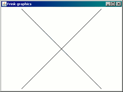
That's it. Frink takes care of the scaling and centering by default. The
coordinates that you choose can be whatever is most convenient and natural
for you. You can also create as many graphics
objects as you
want. By default, when you call graphics.show[]
, each
graphics object is displayed in its own resizable window.
Coordinates
Coordinates in Frink's graphics are very flexible. There are a few things to note:
-
Coordinates are specified as (x, y) with
xbeing the horizontal coordinate andythe vertical coordinate. - Horizontal coordinates increase as you move right.
- Vertical coordinates increase as you move down. (Note that this is the common convention for almost all computer graphics, but is different than the usual mathematical conventions. You can change this using aGraphics Transformation, but be warned that will vertically flip text as well.)
- Arbitrary-sized coordinates: Coordinates can be as big or small as you want. Any real number that Frink can represent is fine.
- Automatic centering and scaling: You don't need to worry about the size or location of your rendering window. By default, all graphics are resized and centered to fit into your graphics device (whether it's a resizable window, a printed page, or a graphic file.) This saves lots of time and effort when drawing most graphics. Even if your graphics have been scaled, translated, and rotated, Frink will still ensure that what you've drawn is scaled and centered.
- Aspect ratio: Aspect ratio is preserved by default. That is, if a rectangle is 2 units wide and 1 unit high, it will retain that shape on resizing. (You can change that by multiplying all coordinates on one axis by a "dummy" dimension that isn't dimensionless and isn't a length.)
- Accurately-scaled drawings : Coordinates may have dimensions of length (e.g. "1 inch"), in which case they are treated specially. In this case, the graphics are still translated to fit into your view window, but Frink will also attempt to render them at the specified size. This is highly dependent on how your operating system reports its resolution. It works very well for printers, but not as well for monitors (especially in Windows, which almost always reports its screen resolution as 96 dpi, no matter what it really is.) This allows you to print exact-sized drawings to the accuracy allowed by your operating system and printer drivers. See the notes below about dimensions.
- Dimensions with units: Including the special case for length, all coordinates can have any units of measure, as long as all coordinates along the same axis have the same dimensions . However, both axes do not have to have the same dimensions as each other, and will be scaled to fit in the window (because preserving aspect ratio is meaningless if they don't have the same units.)
For example, the following short program prints graph paper with a 1 mm grating:
g= new graphics
g.color[.7,.9,.7] //light greenish-gray
for x=0 mm to 8.5 in step 1 mm
g.line[x, 0 in, x, 11 in]
for y=0mm to 11 in step 1 mm
g.line[0 in, y, 8.5 in, y]
g.print[]
Shapes and Colors
All of Frink's graphics are built out of a small number of basic shapes.
These are drawn into a graphics
object using the methods
outlined below. For example, you use them like the following:
g = new graphics
g.color[0,0,0] // black
g.fillEllipseCenter[0,0,10,10]
g.color[1,1,0] // yellow
g.fillEllipseCenter[0,0,9,9]
g.show[]

A new color
object can also be obtained by calling new
color[r, g, b, alpha]
or new color[r, g,
b]
. Note that creating the color this way does not set the
color in any graphics object.
That must be done separately with a
call to graphics.color[c]
.
color[c]
method call.
color[ r, g, b, alpha
]
Also specifies a color, but with transparency. The alpha
component specifies the opacity of the color, and takes values from 0.0 to 1.0, with 1.0 being fully opaque and 0.0 being fully transparent. (Note: transparency requires Java 1.2 or later.) This also returns the color object so you can later re-use it in a color[c]
method call.
color[ colorObject
]
Sets the current color to a color object that has been previously obtained from a call to color[r, g, b, alpha]
, color[r, g, b]
, or a call to the constructor new color[r, g, b, alpha]
or new color[r, g, b]
.
backgroundColor[ r, g, b
]
Sets the background color of the graphics window or image file. The color components are specified as above. There should be only one backgroundColor
method call in a graphics
object, and it should be the first method called when drawing. If more than one call to backgroundColor
is made, this will raise a warning. (It will also replace any existing background color, but that behavior should not be relied on.) By default, the background color is opaque white (or transparent when writing formats like SVG.)
backgroundColor[ colorObject
]
Sets the background color of the graphics window or image file to a color object that has been previously obtained from a call to color[r, g, b, alpha]
, color[r, g, b]
, or a call to the constructor new color[r, g, b, alpha]
or new color[r, g, b]
. The warnings in the above backgroundColor
method also applies to this method.
stroke[ width
]
Sets the stroke width used to draw lines, polygon outlines, ellipses, and polylines. If the width is a dimensionless number, (e.g. 10
) the stroke will be scaled along with the drawing. If the stroke has units of length, (e.g. 2 mm
) the lines will be rendered at that constant width regardless of how the image is scaled. (Note that the stroke width can not be changed in Java 1.1.)
alpha[ opacity
]
Sets the transparency (often called "alpha channel") of all subsequent drawing operations. The opacity is a dimensionless number from 0 (fully transparent) to 1 (fully opaque.) This primarily allows you to draw transparent images, as transparency can already be specified when setting colors. If a color already has a transparency, that transparency value will be multiplied by this global transparency. (Note that the transparency can not be changed in Java 1.1.)
line[ x1, y1, x2, y2
]
Draws a straight line segment between the points (x1, y1) and (x2, y2) using the current color.
fillRectSize[ x, y, width, height
] drawRectSize[ x, y, width, height ]
Draws a rectangle (filled or outlined, depending on the method called) with top left coordinate (x,y) and the specified width and height. If the width or height are negative, this draws the rectangle to the left or to the top of that point. fillRectSides[ x1, y1, x2, y2 ]drawRectSides[ x1, y1, x2, y2 ]
Draws a rectangle (filled or outlined, depending on the method called) defined by its four sides. The sides do not have to be in any particular order. fillRectCenter[ cx, cy, width, height ]drawRectCenter[ cx, cy, width, height ]
Draws a rectangle (filled or outlined, depending on the method called) defined by its centerpoint (cx, cy) and its width and height. fillEllipseSize[ x, y, width, height ]drawEllipseSize[ x, y, width, height ]
Draws a filled or unfilled ellipse (or circle if width==height) with top left coordinate (x,y) and the specified width and height. If the width or height are negative, this draws the ellipse to the left or to the top of that point. fillEllipseSides[ x1, y1, x2, y2 ]drawEllipseSides[ x1, y1, x2, y2 ]
Draws a filled or unfilled ellipse (or circle if width==height) defined by its four sides. The sides do not have to be in any particular order. fillEllipseCenter[ cx, cy, width, height ]drawEllipseCenter[ cx, cy, width, height ]
Draws a filled or unfilled ellipse or circle defined by its centerpoint (cx, cy) and its width and height.Advanced Shapes
Polygons and Polylines
Drawing a curve or a polygon out of line
primitives might not
give good results, as the lines don't know that they're supposed to be
connected to each other. To solve this problem, Frink has polyline
, polygon
and filledPolygon
objects which produce high-quality, connected lines with properly-joined
corners. Drawing a polygon or polyline to a graphics object consists of a
few steps:
-
Create the graphics object (if you haven't done so already.)
g = new graphics -
Create a polygon, filled polygon, or
polyline. (The sample below shows all three. Pick one.)
p = new polygonor
p = new filledPolygonor
p = new polylineAlternately, you can pass in a list of points to any of the above constructors, in which case you can skip the next "adding points" step.
a = [ [1,3], [7,4], [6,2] ] p = new polygon[a]Alternately, you can copy a polygon type to another polygon using the copy constructors:
a = [ [1,3], [7,4], [6,2] ]
p = new polygon[a]
fp = new filledPolygon[p]// copy constructor -
Add an arbitrary number of points to the line or polygon using its
addPointmethod. Each point represents a vertex in the polyline or polygon.
p.addPoint[x,y]
p.addPoint[x,y]
p.addPoint[x,y]Note that a
polygonorfilledPolygonis automatically closed . You should not manually connect the last point back to the first by repeating it at the end of the list. You should only have as manyaddPointcalls as there are vertices in your polygon. -
Add the polygon to the graphics object. A polygon can be added to multiple graphics objects. The drawing color and stroke width used in rendering the polygon are the ones which are active at the time of the
.addcall. Note that no points should be added to the polygon after it is added to the graphics object!g.add[p] -
Show the graphics object (or print, or save it to a file, or keep drawing into it and show it later...)
g.show[]
Polygon Methods
You can call the following methods on a polygon
, filledPolygon
, or polyline
.
cx
, cy
].
getPoints[]
Returns the points in the polygon as an array of [x, y] points.
show[]
Displays the polygon using the default display method.
GeneralPath
A GeneralPath
allows you to create complex shapes consisting
of straight lines, quadratic and cubic Bézier curves, arcs, and
ellipses. These paths can be filled or outlines, and can have multiple
sub-paths that represent the "inside" and "outside" of an object. For
example, rendering a filled letter P
in which one can see
through the "hole" in the P can be obtained with a GeneralPath, and is not
possible with a polygon
.
Note: The GeneralPath functionality is only available under Java 1.2 and later. Attempting to draw with a GeneralPath in earlier releases will produce a warning and the GeneralPath will not be drawn.
Using a GeneralPath
object consists of a few steps:
-
Create the graphics object (if you haven't done so already.)
g = new graphics -
Create a GeneralPath or a filledGeneralPath. (The sample below shows both. Pick one.)
p = new GeneralPathor
p = new filledGeneralPath -
Add an arbitrary number of segments using the following methods on the
GeneralPathclass: Method Description moveTo[ x,y ] Moves to the specified point without drawing. This creates a new subpath. This (oraddPoint[x,y]) should be the first call, otherwise the initial point is unspecified. lineTo[ x, y ] Draws a straight line segment from the current point to the specified point. addPoint[ x,y ] If this is the first point, does amoveTothe specified point. If there are previous points, this does alineTothe specified point. TheaddPointsyntax is retained to make it easy to change code from apolygonorpolylinerepresentation to useGeneralPath.quadratic[ cx, cy, px, py ] Draws a quadratic Bézier curve from the current point to the point specified bypx,pyusing the coordinates specified bycx,cyas the "control point". The curves at each endpoint will be tangent to a line connecting that point and the control point.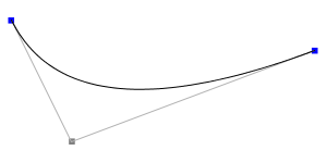
(Control points drawn for clarity.) cubicCurve[ c1x, c1y, c2x, c2y, px, py ] Draws a cubic Bézier curve from the current point to the point specified bypx,pyusing the coordinates specified by (c1x,c1y) and (c2x,c2y) as the "control points". The curves at each endpoint will be tangent to a line connecting that point and its corresponding control point.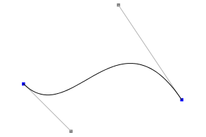
(Control points drawn for clarity.) ellipseSides[x1, y1, x2, y2] Creates an ellipse with the specified coordinates indicating its sides, that is, a rectangle that will contain it. Note that an ellipse is considered to be disconnected from previous line segments, so you should use amoveTo[x,y]after this call to create a new path. ellipseSize[x1, y1, width, height] Creates an ellipse with the (x1,y1) coordinates indicating the top left corner of its bounding box, and the specified width and height relative to that point. Note that an ellipse is considered to be disconnected from previous line segments, so you should use amoveTo[x,y]after this call to create a new path. ellipseCenter[cx, cy, width, height] Creates an ellipse with the (cx, cy) coordinates indicating the center of the ellipse, and the specified width and height. Note that an ellipse is considered to be disconnected from previous line segments, so you should use amoveTo[x,y]after this call to create a new path. circularArc[cx, cy, angle] Creates a circular arc from the current point. The (cx, cy) coordinates indicate the center of the circle, andanglespecifies the angle to go around the circle in the counterclockwise direction. Note that theangleparameter should have units of an angle, e.g.90 degreesor1.2 radiansor even1.2(implying radians) if the standard data file is used which treats radians as a dimensionless number. close[] Closes the current subpath by drawing a straight line to the initial point of the subpath. It is strongly recommended to use this method to close curves, as it properly joins corners, and informs the curve that it is logically closed. This creates a new subpath, so you should use amoveTo[x,y]oraddPoint[x,y]after this call to create a new path. -
Add the GeneralPath to the graphics object. A GeneralPath can be added to multiple graphics objects. The drawing color and stroke width used in rendering the GeneralPath are the ones which are active at the time of the
.addcall. Note that no points should be added to the GeneralPath after it is added to the graphics object!g.add[p] -
Show the graphics object (or print, or save it to a file, or keep drawing into it and show it later...)
g.show[]
For a sample of using the GeneralPath class, see GeneralPathTest.frink which demonstrates drawing a filled letter "P" with a properly-transparent hole.
Graphics with Text
High-quality text with transparent anti-aliased edges can be added
to any graphics
object using the following methods:
font[ fontName, style, height ]
Sets the current font that will be used to render text. The arguments are:
-
fontName: A string indicating the name of the font family. For portability to all platforms and image types (including SVG files,) this should be one of"Serif", "SansSerif", "Monospaced". However, any font name available on your system may be used if you don't care about portability. -
style: An string containing information about the font style. This should contain one of"plain", "bold", "italic", "bold+italic". (It's actually a case-insensitive substring search that just looks for "bold" and "italic" so this can be written in a lot of ways.) -
height: The height of the font in the current coordinate system. Height is taken as the distance from standard baseline to the next standard baseline, not necessarily as the height of the tallest characters. This fits the usual definition of font size used in most systems.If the height is a dimensionless number, (e.g.
10) the font will be scaled along with the drawing. If the height has units of length, (e.g.10 pointsor1 cm) the font will be rendered at that constant height, regardless of how the image is scaled. Note that using a height with dimensions of length might force the text out of the viewable area if the drawing is scaled too small to accommodate it.
If you don't specify a font before drawing text, your system will use its default font, which may give different results when the same program is run on different systems or rendered to different devices. This behavior may change to specify a fixed default font in the future.
text[ text, x, y ] Draws the specified text centered (vertically and horizontally) at the coordinates (x,y). Since it's hard to predict how wide (or tall) text will be until it's rendered, centering is often the most useful option. text[ text, x, y, angle ] Draws text as above, but also rotated by the specified angle (counterclockwise.) The angle must have angular units, ( e.g.90 degrees
or 1 radian
)
text[ text, x, y, horizontalAlign, verticalAlign
]
Draws the specified text with one point specified by the (x,y) coordinates and the rest of the text aligned relative to that as specified by the horizontalAlign
and verticalAlign
parameters.
The parameter horizontalAlign
is a string
containing one of: "left", "right", "center"
indicating if the x
coordinate indicates the left, right,
or center horizontal position of the text. For example, if the
horizontal alignment is given as "right"
, the specified x
coordinate will be the right side of the text.
The parameter verticalAlign
is a string
containing one of: "top", "bottom", "center",
"baseline"
indicating if the y
coordinate indicates
the top, bottom, center, or baseline vertical position of the text. For
example, if the vertical alignment is given as "top"
, the
specified y
coordinate will be the top of the text. The "baseline"
parameter indicates the bottom of most
characters, but characters with descenders like "j", "p" and "q" may
hang below the baseline.
90 degrees
or 1 radian
)
Example: The following program draws a 5x5 grid of random characters.
g=new graphics
g.font["SansSerif", "bold", 10]
for x=1 to 5
for y=1 to 5
g.text[char[random[char["A"], char["Z"]]], x*10, y*10]
g.show[]

Composing Graphics
A graphics
object can be built up from multiple graphics
objects that are added to it. These graphics can be
added at their original size, or placed at a certain location and size.
This makes it easy to create complex graphics from many different graphics
objects that were rendered at their "natural" sizes and then automatically
resized to fit where you want them, no matter what coordinates they
were originally drawn to!
When adding one graphics
obect into another, the new graphics
object added will be transformed according to the current state of theGraphics Transformationand global
transparency (set by the alpha[opacity]
method listed
above in thesection.)
Note that the object is fit according to its estimated bounding box; if the bounding box is estimated too large, then the graphic may not fill the entire region requested, and you may have to manually adjust the scaling.
The following methods on a graphics
object allow you to add
other graphics
objects to them.
See the other add...
methods below to see how to add a
graphic at a specified location and size.
(cx, cy)
and making it fit within the specified width
and height
. This allows you to easily compose a graphics
object out of other graphics
objects, no matter what coordinates they were drawn to.
The aspect ratio of the graphic is maintained unless the optional
argument maintainAspectRatio
is set to false
(default is true
).
addCenter
above, but the graphic is rotated around ( cx,cy
) by the specified angle (e.g. 10 degrees
or 1.3 radians
). Positive angles are clockwise.
addSides[ graphics
, x1
, y1
, x2
, y2
, maintainAspectRatio=true
]
Adds another graphic expression to this graphics object, shrinking it or stretching it to fit into a rectangle with the specified sides. The sides do not have to be in any particular order.
The aspect ratio of the graphic is maintained unless the optional
argument maintainAspectRatio
is set to false
(default is true
).
addSides
above, but the graphic is rotated around the center of its bounding box by the specified angle (e.g. 10 degrees
or 1.3 radians
). Positive angles are clockwise.
addSize[ graphics
, left
, top
, width
, height
, maintainAspectRatio=true
]
Adds another graphic expression to this graphics object, shrinking it or stretching it to fit into a rectangle with top left coordinate (left, top) and the specified width and height. If the width or height are negative, this draws the graphic to the left or to the top of that point, allowing you to align a graphic to the left, right, top, or bottom of a point or line.
The aspect ratio of the graphic is maintained unless the optional
argument maintainAspectRatio
is set to false
(default is true
).
addSize
above, but the graphic is rotated around the center of its bounding box by the specified angle (e.g. 10 degrees
or 1.3 radians
). Positive angles are clockwise.
Transforming Graphics
Frink allows you to rotate, translate, and scale graphics objects, allowing you to write simple code using the coordinate system that is most logical, and translate or scale it wherever you want. Like all of Frink's other graphics, Frink ensures that whatever you draw is automatically scaled and centered into the display, and can be exported to various file formats.
The current graphics transformation can be saved with a call to graphics.saveTransform[]
and should be restored with a
corresponding call to graphics.restoreTransform[]
.
The following methods are available on a graphics
object to
transform the coordinates. Each transform is appended to the previous
transforms. After making a transformation, all subsequent drawing or add[]
commands will use the current transform.
dx
moves to the right, positive dy
moves down.) Technical Note: This corresponds to the matrix multiplication:
x' 1 0 dx x y' = 0 1 dy * y 1 0 0 1 1which gives the equations:
x' = x + dx
y' = y + dy
Scales all subsequent drawing commands around the point (0,0) by the specified scale on the x and y axes. A coefficient of 1 corresponds to no scaling on that axis. A negative coefficient indicates a flip on that axis. (Note that this will also flip text!)
Note that this function is not usually what you need; you usually want to scale around another point. See the four-argument version of this function below.
Technical Note: This corresponds to the matrix multiplication:
x' sx 0 0 x y' = 0 sy 0 * y 1 0 0 1 1which gives the equations:
x' = sx x
y' = sy y
(cx,cy)
by the specified scales sx,sy
on the x and y axes. A coefficient of 1 corresponds to no scaling on that axis. A negative coefficient indicates a flip on that axis. (Note that this will also flip text!)
This is equivalent to the less-efficient:
translate[cx, cy]
scale[sx, sy]
translate[-cx, -cy]
Technical Note: This corresponds to the matrix multiplication:
x' sx 0 cx(1-sx) x y' = 0 sy cy(1-sy) * y 1 0 0 1 1which gives the equations:
x' = sx x + cx (1 - sx)
y' = sy y + cy (1 - sy)
or, equivalently:
x' = sx (x-cx) + cx
y' = sy (y-cy) + cy
Rotates all subsequent drawing commands around the point (0,0) by the specified angle. Positive angles are clockwise.
Note that this function is rarely what you need; you usually want to rotate around another point. See the three-argument version of this function below.
Technical Note: This corresponds to the matrix multiplication:
x' cos[angle] -sin[angle] 0 x y' = sin[angle] cos[angle] 0 * y 1 0 0 1 1which gives the equations:
x' = x cos[angle] - y sin[angle]
y' = x sin[angle] + y cos[angle]
cx, cy
) by the specified angle. Positive angles are clockwise.
This is equivalent to the less-efficient:
translate[cx, cy]
rotate[angle]
translate[-cx, -cy]
Technical Note: This corresponds to the matrix multiplication:
x' cos[angle] -sin[angle] cx (1-cos[angle]) + cy sin[angle] x y' = sin[angle] cos[angle] cy (1-cos[angle]) - cx sin[angle] * y 1 0 0 1 1which gives the equations:
x' = x cos[angle] - y sin[angle] + cx (1-cos[angle]) + cy sin[angle]
y' = x sin[angle] + y cos[angle] + cy (1-cos[angle]) - cx sin[angle]
or, equivalently:
x' = (x - cx) cos[angle] - (y - cy) sin[angle] + cx
y' = (x - cx) sin[angle] + (y - cy) cos[angle] + cy
Performs an arbitrary affine transform on subsequent drawing commands, by specifying all relevant coefficients of an affine transformation matrix. This corresponds to the matrix multiplication:
x' a c e x y' = b d f * y 1 0 0 1 1which gives the equations:
x' = a x + c y + e
y' = b x + d y + f
See the technical notes for the above functions to see how various transformations are achieved by specifying the coefficients of this matrix. Note also that this function can be used to create skews as well as rotations, translations, and scales.
Technical Note: If you want to reverse this transformation, or any of the above transformations, the inverse equations are:
x = (c (f - y') - d (e - x')) / (a d - b c)
y = -(a (f - y') - b (e - x')) / (a d - b c)
saveTransform[]
Saves the current state of the graphics transform so it can later be restored with a call to restoreTransform[]
restoreTransform[]
Restores the state of the graphics transform to the point where the last saveTransform[]
was called.
Clipping Graphics
To constrain the area in which graphics can be drawn, you can specify a
clipping region on a graphics
object. After
you set
a clipping region, subsequent drawing commands will only be drawn within
that region.
A cool thing about the clipping implementation is that, like all of Frink's graphics, you can draw to any coordinate system that makes sense to you, even if it's rotated, scaled, skewed, and clipped, and Frink will automatically center and scale that into your graphics window by default, greatly simplifying many graphics programming tasks. In other words, clipping can be used to "zoom in" on a section of a larger graphic--just set a clipping region before drawing the graphic and only the section within the clipping region will be displayed.
Each time you add a clipping boundary, it narrows the existing clipping boundary, and the clipping boundary will become the intersection of the previous clipping boundary and the new clipping boundary.
Clipping boundaries can be saved and restored with the graphics.saveClip[]
and graphics.restoreClip[]
methods. Currently, these
must be properly nested with graphics.saveTransform[]
and graphics.restoreTransform[]
calls.
The following methods are on a graphics
object.
polygon
, or GeneralPath
. (The new clipping boundary is the intersection
of the old boundary and the new boundary, always making the clipping boundary smaller.)
saveClip[]
Saves the current clipping region so it can later be restored with a call to restoreClip[]
.
restoreClip[]
Restores the current clipping region to the state it had at the last call to saveClip[]
. Currently, these calls must be properly nested with graphics.saveTransform[]
and graphics.restoreTransform[]
calls.
Antialiasing
By default, graphics and text are antialiased on most platforms. That is,
edges of lines and text are smoothed and slightly blurred to reduce jagged
edges. This may be unwelcome in some situations, such as when drawing many
adjacent rectangles. Antialiasing of graphics and text can be controlled
by the following methods on a graphics
object.
false
, all subsequent shape drawing operations to that graphics
object will no longer be anti-aliased. (Note that this does not affect anti-aliasing of text, which is controlled separately by the antialasedText
function below.) This may be turned on and off over the course of drawing a single graphics
object. Not all graphics environments support control of anti-aliasing, as noted below: -
SVG
: The SVG specification does not directly allow control of antialiasing, but Frink sets the
shape-rendering="crispEdges"rendering property (link opens in new window), which seems to turn off antialiasing in many rendering environments. - HTML5 : The HTML5 canvas specification does not seem to allow any control of antialiasing, so this does nothing.
false
, all subsequent text drawn to that graphics
object will no longer be anti-aliased. This may be turned on and off over the course of drawing a single graphics
object. Not all environments support control of anti-aliased text, as noted below: -
SVG
: The SVG specification does not directly allow control of antialiasing, but this sets the
text-rendering="optimizeSpeed"rendering property (link opens in new window), which seems to turn off text antialiasing in many rendering environments. - HTML5 : The HTML5 canvas specification does not seem to allow control of antialiasing, so this does nothing.
Showing Graphics
Once a graphics
object has been constructed, it can be shown
on-screen, printed, or written to a file using the following methods:
insets
is a floating-point value between 0 and 1, where 1 means to use 100% of the window with the graphic (no borders.) An insets value of 0.95 causes 95% of the window's width and/or height to be graphics, and 5% as borders. These insets are in addition
to any margins you set in the print dialog. (Specifying insets is usually only necessary when rendering a background color that you want to have extend a certain distance around the graphic.)
printTiled[ pagesWide, pagesHigh
]
Prints the graphics object tiled across multiple pages on a printer. This allows very large graphics to be printed. The arguments indicate how many printer pages wide and high the graphic should be drawn.
printTiled[ pagesWide, pagesHigh, insets
]
Prints the graphics object tiled across multiple pages on a printer. This allows very large graphics to be printed. The arguments indicate how many printer pages wide and high the graphic should be drawn. insets
is a floating-point value between 0 and 1, where 1 means to use 100% of the window with the graphic (no borders.) An insets value of 0.95 causes 5% of the window's width and/or height to be borders. These insets are in addition
to any margins you set in the print dialog. (Specifying insets is usually only necessary when rendering a background color that you want to have extend a certain distance around the graphic.)
invertGrays[]
Takes a graphics
and returns a new graphics
object in which the black colors are turned to white and the whites are turned to black, with all the colors near to gray inverted the same way. This does not affect other colors; red remains red. This is useful for making graphics that look like Wargames on-screen (black background with white lines) but don't destroy your printer ink budget. A typical usage would be:
// Draw default graphics which are black on white background
g.invertGrays[].show[] // Make it look like Wargames on screen
g.print[] // Don't use up my printer ink, Joshua
data
URI, included in an email, etc.
write[ filename, width, height
] writeTransparent[ filename, width, height ]
write[ filename, width, height, insets ]
writeTransparent[ filename, width, height, insets ]
Writes the image to a file with the specified width and height (usually in pixels). The format of the file is guessed from the filename's extension. If thewriteTransparent
method is called, and if the image format supports it, the image will be rendered with a transparent background, allowing you to stack and create composite images with full anti-aliasing and background support.
If exactly one of width
or height
are
specified as undef
, the size of the undefined axis will be
calculated from the defined width or height and the aspect ratio of the graphics
that is being drawn.
In the versions of these functions where insets
is
specified, the value of that argument indicates how wide a border
should be left when drawing. When specifying 1
(indicating
100%) to the insets
argument, the drawn image occupies
100% of the width and height, with no border. By default, only 95%
(0.95) of the width or height is used, leaving a small 5% border around
the drawn graphics. Specifying the insets is important when rendering
image files out at their original size. See thesection of the documentation for more.
The file formats supported by your version of Java may vary, but the following should be supported:
- JPEG : Does not support transparency. Requires Java 1.4 or later.
- PNG : (Portable Network Graphics) Supports transparency and full anti-aliasing of transparent graphics. Requires Java 1.4 or later.
- SVG : (Scalable Vector Graphics) A vector format that is infinitely resizable. Supports transparency. By default, all backgrounds in SVG graphics are transparent. Works in all versions of Java. Warning: Due to a deficiency in the SVG standard, drawings with dimensions of length (e.g. "1 inch") may not work properly for some shapes, notably polygons, polylines, and GeneralPath.
- SVGZ : (Scalable Vector Graphics, compressed with GZIP) This is the same as the SVG format, but is compressed with the GZIP compression algorithm. Since SVG files usually contain a lot of repetition, using this format will significantly reduce file size and should be parseable by most/all programs that can handle SVG files.
-
: (HTML5 canvas support required) While HTML5 will not be a finalized specification until at least 2014, major modern browsers for desktop and mobile devices (Firefox, Chrome, Opera, Safari, IE) support the HTML5 features that Frink requires.
- Transmission of vector graphics in vector formats, allowing efficient, antialiased rendering of vector graphics.
-
Bitmapped images are transmitted within the HTML document as embedded
dataURIs encoded in base-64, allowing you to send the entire graphic as a single HTML file. Bitmapped images are transmitted at the end of the file, and displayed as they are loaded, allowing progressive display of documents containing multiple bitmaps. -
All of Frink's graphics primitives are supported, including bitmaps,
GeneralPath, partially-transparent graphics, rotations, translations, and scaling. - HTML5 is rendered to relatively simple, user-modifiable code.
-
What doesn't work in HTML5 (future wish list):
-
Drawings with dimensions ( e.g.
a rectangle with width
1 inch) does not get rendered properly to HTML5. I'm still doing research to see if we can get a reasonable resolution figure from the rendering environment. -
HTML5, for some ungodly reason, for a long time did not not support the even-odd
winding rule
for filling graphics, which becomes important when drawing an arbitrary
GeneralPathand self-intersecting or concentric filled polygons. HTML5 only supported the rather stupid and useless nonzero winding rule which will make some objects with "hollow" centers not render the same in HTML5 as they do in all other sane environments (e.g. Swing, AWT, Android, SVG, PostScript, PDF).However, this problem is being gradually addressed in current browsers, (but not yet in the official HTML5 Canvas spec !) but your browser needs to support the HTML Canvas's
context.fill("evenodd")method for Frink's graphics to work properly now. This appears to be supported in current versions of Firefox (21+), Firefox on Android, Chrome (27+), Opera (15+), Safari 8.0, and IE11 ( according to this ). - Animation is not yet possible in HTML5. It's not clear if this will be easy without porting all of Frink to JavaScript.
- All bitmapped graphics are embedded in PNG format. These may be larger than the corresponding JPEG graphics, but they are lossless and allow alpha channels, which JPEG does not allow. It's possible that there may be a switch in the future to embed bitmaps in JPEG format and to control the quality, or the renderer may get "smarter" and determine if alpha channels are present, and switch rendering formats for efficiency.
- When rendering just a portion of a bitmapped image to HTML5, the entire original bitmap file is transmitted in the HTML5 document.
-
If the browser doesn't support the HTML5
canvaselement, Frink could theoretically render a small thumbnail image (or full-resolution image, but that would be wasteful) showing the user what they're missing. If the browser doesn't supportcanvas, the user is warned about possibly needing to open the document in a newer browser. - There appears to be no way to controlin the HTML5 spec
-
Drawings with dimensions ( e.g.
a rectangle with width
writeFormatTransparent[ filename, format, width, height ]
Writes to a file, explicitly specifying the format. The format should be a string containing one of"svg", "SVG", "svgz", "SVGZ", "jpeg", "JPEG", "jpg", "JPG", "png", "PNG", "html", "HTML"
, or possibly another format that your platform understands (like " webp
" / " WEBP
" on Android.)
The following draws a partially-transparent circle, and then successively displays it on-screen, prints it, and renders it to various image files:
g = new graphics
g.color[0, 0, 1, 0.5] // Blue,
half-transparent
g.fillEllipseCenter[0,0,10,10]
g.show[]
g.print[]
g.write["circle.jpg", 200, 200]
g.write["circle.png", 200, 200]
g.writeTransparent["circleTrans.png", 200, 200]
g.write["circle.svg", 200, 200]
g.write["circle.html", 200, 200]
Graphics Functions
Function Description getBoundingBox[ graphicsExpression ] Returns the coordinates of the bounding box for the graphics object in the form[left, top, right, bottom]
. If the bounding box is empty (that is, there are no drawable elements in graphicsExpression
, this returns undef
.
Images
Bitmap images can be loaded and drawn to a graphics object, displayed in their own window, resized, printed (including tiled across several pages,) drawn over, saved out to files, etc. You can also load an image or create it in memory, and read or write the values of individual pixels, allowing image processing or analysis.
Note that Java 1.1 and earlier did not have a portable, public way to read and write individial pixels of images, so many of these methods require Java 1.2 or later.
To load an image, call new image[URL]
, passing it a
URL. The URL can be of any type your Java platform understands, including a file:
URL indicating a file on your local system:
img1 = new image["http://futureboy.us/images/futureboydomethumb4.gif"]
img2 = new image["file:yourfile.gif"]
An image can also be loaded from a Java object that contains an
already-opened java.io.InputStream
: new
image[java.io.InputStream]
. This allows you to create images
from open files, URLs, network sources, servlet containers, in-memory
sources, etc., without writing their data to temporary files.
To create a new (blank) image, specify the width and height in pixels:
img3 = new image[640, 480]
To copy an image, use the copy constructor:
img4 = new image[img3]
This will make a copy of all of the pixels in the image, so the copy can be modified without modifying the original.
You can turn a graphics
object into a bitmapped image in
memory by using the constructor:
new image[graphics, width, height]
Where width
and height
are dimensionless
integers. This gives you a readable/writable bitmap which allows you to
read and write the individual pixels of the graphic. For example, to
create a graphic and then render it to a bitmapped image in memory, you may
do something like:
g = new graphics
g.line[0,0,1,1]
img4 = new image[g, 300, 300]
Note that there are already methods to write graphics to a bitmapped file format. Using this constructor is only necessary if you want to read or write specific pixels of the rendered graphic directly in memory .
The image can be then shown in its own window by calling the .show[]
method:
img1.show[]
The following table summarizes the methods available on an image
object:
[width, height]
. You can thus call it like: [width,height]=image.getSize[]
getPixel[x,y]
Returns the pixel's color as an array of [red, green, blue, alpha] components between, each between 0 and 1 inclusive.
getPixelInt[x,y]
Returns the pixel's color as an array of [red, green, blue, alpha] components between, each between 0 and 255 inclusive.
getPixelAsColor[x,y]
Returns the pixel's color as a color
object that can be passed to other methods that take color objects.
setPixel[x, y, red, green, blue, alpha]
Sets the specified pixel's color to the color specified by the red, green, blue, alpha components, each between 0 and 1 (inclusive).
setPixel[x, y, red, green, blue]
Sets the specified pixel's color to the color specified by the red, green, blue, components, each between 0 and 1 (inclusive). The pixel will be fully opaque.
setPixelInt[x, y, red, green, blue, alpha]
Sets the specified pixel's color to the color specified by the red, green, blue, alpha components, each between 0 and 255 (inclusive).
setPixelInt[x, y, red, green, blue]
Sets the specified pixel's color to the color specified by the red, green, blue, components, each between 0 and 255 (inclusive). The pixel will be fully opaque.
setPixel[x, y, color]
Sets the specified pixel's color to a color designated by the color
object.
averagePixels[left, top, right, bottom]
Returns the average color of the pixels within the region specified by the given coordinates. Each coordinate may be a floating-point value, and if an incomplete pixel is sampled, it is weighted accordingly. The return value is an array of [red, green, blue, alpha] components, each between 0 and 1 inclusive. The values for the coordinates can range from 0 to ( im.getWidth[]
or im.getHeight[]
,) inclusive, indicating, for example, the left and right side of the pixel (or subpixel) to be sampled. For example, in a 2x2 pixel image, you'd want to sample [0,0,2,2] to average the whole image.
makeARGB[]
Forces a loaded image to have an ARGB color model, that is, to have an 24-bit true color model with an 8-bit alpha channel that supports transparency. By default, when loading an image, the color model is preserved and may not support true color nor transparency.
makeMono[]
Forces a loaded image to have a one-bit monochrome color model, if your platform supports it. This may perform dithering on the image. For Android : Currently, the Android Bitmap.Config class does not support monochrome images, so this does nothing on Android.
write[ filename ] - Write the image to the specified filename. The format of the file is guessed from the filename's extension. The file formats supported by your version of Java may vary, but the following should be supported:- JPEG : Does not support transparency. Requires Java 1.4 or later.
- PNG : (Portable Network Graphics) Supports transparency and full anti-aliasing of transparent graphics. Requires Java 1.4 or later.
data
URI, included in an email, etc.
toComplexArray[]
Turns the bits of the image into a 2-dimensional array of complex values, which can be transformed quickly with thefunctions. The behavior of this method will probably change.
toComplexArrayFromLog[ center=false
]
Assumes that this image contains magnitude and phase information (green encodes magnitude, red encodes phase) of a logarithmically-encodedFourier
transformof an image, and reconstructs a 2-dimensional ComplexArray2D
with the values from the image. In other words, this is the inverse of ComplexArray2D.toLogImage[decenter=false]
. The behavior of this method will probably change. See the sample program
FourierImage.frinkfor a sample of FFT transforming an image, writing it as a log-encoded
image, reading it back, and inverse-transforming back to the original
image.
show[]
Displays the image (by default, in its own
window.)
show[ title
]
Displays the image (by default,
in its own window) with the specified title.
print[]
Prints the image to a printer.
print[ insets
]
Prints the image to a
printer. insets
is a floating-point value
between 0 and 1, where 1 means to use 100% of the window with the graphic
(no borders.) An insets value of 0.95 causes 5% of the window's width
and/or height to be borders. These insets are in addition
to any margins you set in the print dialog.
printTiled[ pagesWide, pagesHigh
]
Prints the
image to a printer, tiled across several pages to make a very large
image.
printTiled[ pagesWide, pagesHigh,
insets
]
Prints the image to a printer, tiled across several
pages to make a very large image. insets
is a floating-point value
between 0 and 1, where 1 means to use 100% of the window with the graphic
(no borders.) An insets value of 0.95 causes 5% of the window's width
and/or height to be borders. These insets are in addition
to any margins you set in the print dialog.
resize[ width, height
]
Resizes an image to
the new specified width and height and returns a new image. It does not
modify the original image. If either width
or height
are the special value undef
or 0
, then one dimension is constrained and the other
dimension is calculated to preserve the aspect ratio of the original
image.
Drawing images into graphics
Images can be drawn onto a graphics
object with the following
methods on the graphics
object:
graphics
object with the specified top left coordinates and the specified width and height. Note that this method does not
specifically preserve the image's aspect ratio and thus may distort the image if the width and the height are not in the same ratio as in the original image. To preserve the aspect ratio automatically, use one of the methods below.
draw[ image, left, top, width, height, leftSrc, topSrc, rightSrc, bottomSrc
]
Like draw
above, but draws part
of the specified image. The parameters ending in Src
contain the pixel values of the image to include. To preserve the aspect ratio automatically, use one of the methods below.
fitCenter[ image, cx, cy, width, height
]
Draws an image onto the graphics
object with the specified center coordinates (cx,cy), making it fill the specified width and height as much as possible without modifying the aspect ratio.
This will thus preserve the proportions of the image.
fitCenter[ image, cx, cy, width, height, leftSrc, topSrc, rightSrc, bottomSrc
]
Like fitCenter
above, but draws part
of an image. The parameters ending in Src
contain the pixel values of the image to include.
fillCenter[ image, cx, cy, width, height
]
Draws an image onto the graphics
object with the specified center coordinates (cx,cy), making it completely fill the specified width and height without modifying the aspect ratio. Note that this may cut off part of the image!
fillCenter[ image, cx, c,y width, height, leftSrc, topSrc, rightSrc, bottomSrc
]
Like fillCenter
above, but draws part
of an image. The parameters ending in Src
contain the pixel values of the image to include. Note that this may cut off part of the image!
See therewriteImage.frink sample program for an example of loading an image, writing a semi-transparent watermark over it, and then saving the image out to another file at its original size.
Animation
Animation is performed by calling
the replaceGraphics[g]
method on a graphics window
(obtained by graphics.show[]
) which replaces the
graphics object with a new graphics object and repaints the window.
A short sample of animation is available in theanimate.frink sample program.
An on-screen graphics window can be repainted as items are added to
its graphics
object. Repainting is not done automatically,
but is under the programmer's control. This allows the screen to be
repainted only when desired.
The graphics.show[]
method returns an object with a repaint[]
or replaceGraphics[g]
method
that instructs the graphics window to be painted. Tip:
don't save
this object if you're not planning on doing incremental animation, or set
the variable to some value such as undef
when animation is
complete. This will allow the window's resources to be garbage-collected
as soon as possible.
g = new graphics
window = g.show[]
for x = 1 to 10
{// Do something that takes a long time...
g.fillRectCenter[x,0,1,1]
window.repaint[]
}
Animated Images
Frink can combine a series of graphics
objects into a single
animated GIF image very simply. The series of steps is:
-
Create an object of type
Animation, optionally setting the frame rate. The frame rate can be specified as either a time or a frequency, for example,1/30 sor33 msor30/s.
a = new Animationor
a = new Animation[30/s] -
Create a
graphicsobject for each frame and draw into it using the methods described above.
g = new graphics
...drawing code goes here... -
Add the
graphicsobject to theAnimationobject using itsaddmethod:
a.add[g] - Repeat steps 2 and 3 for each frame of your animation.
-
Write the animated image to a file at any resolution using the
Animation.write[filename, width, height]method:
a.write["animation.gif", 400, 400]
Animated Image Methods
Method Description add[ graphics ] Adds a new frame to the animation, represented by thegraphics
object. This may also be an image
.
write[ filename, width, height
] write[ filename, width, height, insets ] Writes the animation to the specified filename. Currently, no matter what filename is specified, the format will be an animated GIF.
width
and height
are integers. If the insets are specified, they must be a number between 0 and 1 indicating how much of the image is filled by the graphics. If insets
is 1, the graphics will fill the entire image with no border.
toBase64[ width, height
]
Turns the animation into a base-64 encoded string in animated GIF format.
Sample Graphics Programs
Below is a small list of simple but interesting and powerful programs that demonstrate Frink's graphics.
Filename Description animate.frink Demonstrates simple animation. graphpaper.frink Prints graph paper with 1 cm and 1 mm grids. Demonstrates exactly-sized printing. rewriteImage.frink Loads a bitmap image and writes a semi-transparent watermark on it and then saves it back out to a file. Demonstrates image loading, drawing over images, and saving image files at their original size. SolarCooker2.frink Draws a parabola and focal point for a small solar cooker that you can cut out and use to make a precisely-shaped mirror for cooking hot dogs and such. simplegraph3.frink A very powerful but simple program to graph just about any equation, no matter how complicated or ill-behaved, using Frink'scapabilities. spiral.frink Draws simple, colorful spirals. Fiddle with the numbers to make different, interesting patterns. drawSolarSystem.frink Draws the current position of planets in the solar system. (With exaggerated scale, otherwise they're invisible.) Requires theplanets.frink andsun.frink libraries.Temperature Scales
Temperature scales that have their zero point (kelvin, Rankine) at absolute zero can be multiplied and converted normally.
45 Rankine -> K
25
Temperature scales like Fahrenheit, Celsius, and Reaumur cannot be
represented as normal multiplicative unit definitions because their zero
point is not at absolute zero.
Thus, to avoid ambiguous "do what I mean" interpretation, you must use the
functions Fahrenheit[x]
or the shorter F[x]
, Celsius[x]
or the shorter C[x]
, and Reaumur[x]
to convert to/from these
temperature scales:
To represent a Fahrenheit temperature:
Fahrenheit[451]
or
F[451]
505.9277777777778 K (temperature)
To convert another temperature scale to Fahrenheit:
Fahrenheit[30 K]
or
F[30 K]
-405.67
To represent a Celsius temperature:
Celsius[0]
or
C[0]
273.15 K (temperature)
To convert another temperature scale to Celsius:
Celsius[30 K]
or
C[30 K]
-243.15
To convert between scales (short version):
Fahrenheit[98.6] -> Celsius
or
F[98.6] -> C
37.0
This is equivalent to saying:
Celsius[ Fahrenheit[98.6] ]
or
C[ F[98.6] ]
Except this way doesn't
turn the result into a string like the ->
operator does.
Note:
The units degC
and degF
only
indicate the difference in the size
of a degree in these various
scales. They should only be used when you're indicating the difference
between two temperatures, (say, how much energy to
raise the temperature of a gram of water by 5 degrees Celsius,) not
for absolute temperatures. Conversely, the conversion
functions above should not
be used when the difference
between temperatures in two scales should be compared.
The International System of Units (SI) considers the thermodynamic
temperature in kelvin and the size of a degree in the kelvin system to have
the same units. See Resolution 3 of the 13th CGPM
(1967/68)
. This means that you can use K
as either an
absolute thermodynamic temperature, or a temperature difference. However,
this implies that Frink can't automatically guarantee that "do what I mean"
calculations with temperature are correct, as it would have to magically
guess what you mean.
Other Data Sources
One of the main design goals of Frink was to allow new sources of data to be added in very easily. These special sources are not necessarily defined in thedata file. The three data sources listed below retrieve data on demand from up-to-the-minute data on the Internet (and thus require connection to the Internet.)
Historical U.S. Price Data
Obligatory Disclaimer: This feature requires connection to the internet. If you are using Frink on a handheld device, you may incur connection charges. Also, since I cannot guarantee the availability of any internet sites, this feature is intended only as a bonus that may not work reliably if at all. You may also require someif you use an FTP proxy server to access the web.
The units "dollar" or "USD" indicate the value of a current U.S. dollar (which is arbitrarily chosen as the standard unit of currency.) Historical price data is available to allow comparisons between the historical "buying power" of U.S. currency. This allows you to adjust historical prices for inflation. These are represented by specially-named units containing both the currency and the year, separated by an underscore, for example:
- 1.25 dollar_1960
- dollar_1902
- dollars_1902
- 10 dollars_1902
- 10 USD_1902
- cent_1910
- 5 cents_1926
- cent_1914
Data after 1913 is fetched live from the U.S. Department of Labor Bureau of Labor Statistics Consumer Price Index data, specifially by retrieving and parsing this file . If that file is unavailable, the data will be fetched from a static file distributed with Frink, which is only as recent as your version of Frink.
Since the U.S. Department of Labor Bureau of Labor Statistics no longer maintains a machine-readable Consumer Price Index file, the file is fetched from the St. Louis Federal Reserve, specifically by parsing this file. The new data is also cached in each Frink jar file in case you don't have network connectivity.
Data from 1700 to 1912 is based on some general economists' guesses and should be taken with a grain of salt. U.S. data before 1700 is not available, and probably wouldn't be meaningful unless you could convert between the value of pelts, tinder, and tallow.
Warning: The BLS web and FTP servers seem to have frequent outages, and historical data will not be available if the servers are down, or if you are not connected to the Internet. Frink contains an internal cache of the CPI data in this case.
From 1913-present, you can even use monthly resolution by indicating the month after the year. Months are 2 digits and padded with zeros:
- dollar_1969_08
- dollars_1969_08
- 14.75 dollar_1941_12
- 14.75 USD_1941_12
- dollars_1941_12
- dollar_1941_12
- 15 cents_1965_10
- 4 cent_1929_01
Historical currency values can be converted to the current value. For example to find today's cost of Mark Twain's passage to Europe and the Holy Land on the steamship Quaker City at a cost of $1250 in 1867 (detailed in The Innocents Abroad , the conversion of which was one of my first web projects):
1250 dollar_1867 -> dollar
14982.240769251547535000
And, you can add the 5 dollars/day in gold that they were encouraged to bring along to cover expenses for the 6-month trip:
1250 dollar_1867 + 5 dollars_1867/day 6 months
-> dollar
26043.38587544437
You can translate from one year and month to another, if you have a DeLorean, and want to watch a Reagan movie:
50 cents_1955_11 -> dollars_1985_10
2.020446096654275
Historical British Price Data
The units Britain
or Britain_Pound
or Britain_currency
or Great_Britain
or Great_Britain_Pound
or United_Kingdom_Pound
, or England
or England_currency
or GBP
(the ISO-4217
code for the U.K. Pound) indicate the current
pound (but don't use pound
by itself--that's a measure of mass.) The exchange rate
between the pound and all other world currencies, see below, is fetched
live from the Internet.
Historical price data is available to allow comparisons between the historical "buying power" of British currency, both pre- and post-decimalization. Data goes back to the year 1245. I don't know if data before this would be very meaningful.
Historical currency values are represented by specially-named units
containing both the currency and the year, separated by an underscore. All
can be used in the plural, ( e.g.
pound_1960
or pounds_1960
or GBP_1960
are all valid). The
following are examples of the plethora of values up to and including 1970
(from 1971 on, it just became pounds and pence):
No wonder they went to decimalization. It was either that or go to base-960 math.
To form combinations you can add them (using parentheses when necessary). For example, to convert a historical rate per day to current dollars/year:
(4 pounds_1860 + 3 shilling_1860 + 5 pence_1860) / day
-> dollars/year
101853.3826649
I acknowledge that's a bit cumbersome.
So, you can find out what a great amount of money was involved when the British Parliament announced a 20,000 pound prize in 1714 for solving the Longitude Problem :
20000 pound_1714 -> dollars
2807866.8
That's a lot of lettuce. For more about the fascinating history of this problem, I highly recommend Dava Sobel's Longitude: The True Story of a Lone Genius Who Solved the Greatest Scientific Problem of His Time . By God, Harrison, I will see you righted.
Thanks to Dan Weiler who loaned me the above book which I never returned (and passed along to my Grandpa.) Sorry, Dan, I'll buy you a book of your choice.
International Exchange Rates
Obligatory Disclaimer: This feature requires connection to the internet. If you are using Frink on a handheld device, you may incur connection charges. Also, since I cannot guarantee the availability of any internet sites, this feature is intended only as a bonus that may not work reliably if at all. Java versions 1.6 and before may not be able to use this due to cryptography limitations. You may also require someif you use an HTTP proxy server to access the web.
Current exchange rate between almost all of the world's currencies is available. Exchange rates are fetched live from an allegedly zero-delay source on the Internet. The currency can either be specified by the name of the country, by the 3-letter ISO-4217 code for the currency, or by one of the combinations shown below. The following examples all work:
- Ireland
- Ireland_currency
- Ireland_Punt
- IEP
- Japan
- Japan_currency
- Japan_Yen
- JPY
- yen (this works because only Japan has a currency called "yen")
- Yen
- United_Arab_Emirates
- United_Arab_Emirates_currency
- United_Arab_Emirates_Dirham
- AED
- Euro
- EUR
To list all of the currencies, you can use:
units[currency]
So, I'm watching "The Amazing Race" and seeing a team pay 600 Baht in Thailand for a hotel room. How much is that in a currency I'm familiar with?
600 baht -> USD
13.73724
I could have also used Thailand_Baht
or Thailand
in the above example.
You can also get the current trade rates of various precious metals (normalized from the obscure troy weights that these values are measured in.) These are referenced using the capitalized name (lower case brings up element properties for now... this will all be addressed when I add object-oriented behavior to Frink) or the 3-letter ISO code (which is an X followed by the chemical symbol):
Element ISO Code Gold XAU Platinum XPT Silver XAG Palladium XPD
Gold
8765.9010519364188896 kg^-1 USD (price_per_mass)
Note that this is in units of currency/mass (the international exchange rates for these are specified in dollars/troyounce, (but try to find that written somewhere)), but you can use any units of mass you want:
1 ton Gold
7952291.666666666667 USD (currency)
Or find out how much it would be worth to melt down that necklace:
3 gram 18 karat Gold
19.723277366856942501600 USD (currency)
Note: If you want to set a different base currency in your units file, and if you want currency conversions to still work, you should now) define the base currency as its 3-letter ISO-4217 currency code (say, "EUR" or "JPY"). This will allow the currency converter to unambiguously figure out which currency you mean. The following special cases work as well:
Symbol Description dollar U.S. dollar Euro Euro euro euro € Euro symbol (Unicode\u20ac
)
¥
Japanese Yen symbol (Unicode \u00a5
)
£
U.K. Pound symbol (Unicode \u0163
)
Interval Arithmetic
Frink has the magical ability to perform rigorous interval arithmetic throughout calculations. So what is interval arithmetic? Well, you can think of it as a "new kind of number" that represents a fuzzy range of values. For example, you may know that a value lies between 1 and 2, but you're not quite sure where the value lies in that interval. Depending on your philosophy, you can think of an interval as specifying a fuzzy error bound, or you can think of an interval as simultaneously taking on all values within its bounds.
Frink can take this uncertain interval and propagate the uncertainty through its calculations, giving you the ability to see how the initial uncertainties in your values affect your final calculations.
Currently, the way to indicate that something is an interval is to use the new interval
syntax (although something more concise will
likely be added later, and the output format may change.)
a = new interval[2,3]
b = new interval[5,7]
The intervals can then be manipulated in mathematical expressions, either with ordinary scalar variables or other intervals:
a * 3
[6, 9]
a + b
[7, 10]
a * b
[10, 21]
Intervals may also have a "middle" or "main" value which indicates the best-known value. Note that values should be specified in increasing order.
d = new interval[2, 2.5, 3]
e = new interval[7, 8.2, 9.4]
d * e
[14, 20.5, 28.2]
Of course, all intervals used in a calculation must have "main" values or the main value will be dropped, creating an interval with only upper and lower bounds.
Note: The boundaries and "main" values for intervals must be real numbers. (These numbers can also have dimensions like feet, meters, etc.) Although there is a theory of complex intervals, it's much harder and may not get implemented any time soon, (although a very generous Frink user sent a copy of a rare $200 textbook on complex interval arithmetic which will help that situation! Thanks, Joshua!)
Lest you think that intervals are simpler than they are, I find that people better understand them when they consider the following case:
x = new interval[-2,2]
Now, let's square x. Note that the values at each endpoint are equal to 4. However, over the range [-2,2], the value of x 2 ranges from 4, down to 0 (at x=0), and back up to 4. Frink does the right thing for the values over this whole range:
x^2
[0, 4]
Yeah, that is cool. Frink tracks appropriate boundaries for intervals throughout all of your calculations.
Frink's interval arithmetic is also rigorous in its treatment of error bounds. It painstakingly controls the rounding direction of arithmetic operations so that the boundaries are guaranteed to include the next-largest or next-smallest representable floating-point number that contains the interval. (See notes below onimplementation status.) This is subtle, but I have spent a lot of work ensuring that the boundaries came out trustable, and no bigger than need be. For example:
m = new interval[3,6]
1.0/m
[0.16666666666666666666, 0.33333333333333333334]
Note that the bottom bound is rounded down, and the top bound is rounded up.
Currently, almost all functions have been made interval-aware. Implementing all functions to arbitrary precision will take quite a bit of effort. Of course, that would be much slower, too. Error bounds are unfortunately not "sharp" for all operations (meaning as tight as they could possibly be with limited precision.) I've noted them as such in theInterval Arithmetic Statussection below.
Not all operators such as < > =
make unambiguous sense
when applied to intervals, so Frink has introduced new operators to
disambiguate these cases, and will implement other operators to work with
intervals. See theInterval
Comparison Operatorssection below for more details.
By default, degenerate intervals which have the same upper and lower bounds
are "collapsed" into a single real number. If you want to maintain them as
intervals, call the function collapseIntervals[false]
before
constructing or performing mathematics on those intervals.
As everyone uses Interval Arithmetic for the first time, they come upon two characteristic problems in the field: the dependence problem and the overestimation problem. These are common to all interval analysis, and not just to Frink, and are covered in extensive detail in the Interval Arithmetic section of the Frink FAQ.
For more information about the field of Interval Arithmetic, please visit the Interval Computations website. (Link opens in new window.)
Interval Arithmetic Example
Interval arithmetic is an incredibly powerful feature that allows programs that weren't necessarily written with intervals in mind to track error bounds throughout your calculations, and can be magically applied to programs that are already written. For example, let's take some calculations to find the volume and density of a sphere:
circumference = eval[input["Enter circumference of a sphere: "]]
mass = eval[input["Enter the mass of the sphere: "]]
diameter = circumference / pi
radius = diameter / 2
volume = 4/3 pi radius^3
density = mass / volume
println["The density is: " + (density -> "g/cm^3")]
Now, you can run the program and enter something like "9.1 inches" for the circumference and "5.1 ounces" for the mass and find out the density of your baseball. No surprises there. But when you read the rules of Major League Baseball, you'll find that section 1.09 states:
"The ball shall be a sphere formed by yarn wound around a small core of cork, rubber or similar material, covered with two stripes of white horsehide or cowhide, tightly stitched together. It shall weigh not less than five nor more than 5 1/4 ounces avoirdupois and measure not less than nine nor more than 9 1/4 inches in circumference."
So, using your exact same program above, and a little interval input, Frink can calculate the effects of these allowed variations and show you the allowed range of densities of any legal baseball:
Enter circumference of a sphere:
new interval[9, 9+1/4] inches
Enter the mass of the sphere:
new interval[5, 5+1/4] ounces
The density is: [0.64720283343427980773,
0.73778085086685322066] g/cm^3
The output indicates the range of uncertainties. Note that two different intervals were used to perform this calculation, and the effects of their uncertainties was automatically tracked throughout all calculations. All this in a program that wasn't even written with intervals in mind. Unscrupulous teams may also not that the official definition allows for a large variation in allowable densities of baseballs, which could be manipulated to your advantage.
Also note that I put the units of measure (e.g. inches, ounces) outside the brackets. You could put them inside the brackets, but you'd just have to write them twice in this case. Intervals can, of course, contain units of measure.
By the way, I'm working on a more concise notation for specifying intervals.
Interval Comparison Operators
The relational operators (e.g. < == >
, etc) work with
intervals, but there are many ambiguous cases. These operators try to Do
The Right Thing when applied to intervals. If you compare intervals that
do not overlap, they return the appropriate result. If, however, the
intervals do
overlap, they terminate the program with an error
similar to the following:
Comparison expression: Using operator > to compare intervals [1, 3] and [2, 4] This operator is only defined if there is no overlap between intervals. Please modify your program to use interval-aware comparison operators.
To handle the overlapping cases, Frink defines operators like "certainly
less than" ( CLT
) and "possibly less than" ( PLT
).
These operators can directly replace the normal relational operators.
These new operators also work with normal real numbers, so you can still
write programs that run using either intervals or real numbers as input.
Example:
a = new interval[1,3]
b = new interval[2,4]
a PLT b
true
a CLT b
false
Interval Arithmetic Status
As noted above, not all functions are implemented for intervals. The following table notes the status of the implementation of various operators and functions. If a function does not appear on this list, it may still return values for interval arguments, but you shouldn't trust it because I haven't evaluated it for discontinuities or non-monotonicity yet.
Function / Operator Arbitrary Precision? Rigorous Error Bounds? Notes + Y Y - Y Y * Y Y / Y Y mod Y Y ^ N N Performed to hardware precision only. floor[ x ] Y Y ln[ x ] N Y Performed to hardware precision only. log[ x ] N N Performed to hardware precision only. exp[ x ] N Y Performed to hardware precision only. sin[ x ] N N Performed to hardware precision only. cos[ x ] N N Performed to hardware precision only. tan[ x ] N N Performed to hardware precision only. sec[ x ] N N Performed to hardware precision only. csc[ x ] N N Performed to hardware precision only. cot[ x ] N N Performed to hardware precision only. arccos[ x ] N Y Performed to hardware precision only. arcsin[ x ] N Y Performed to hardware precision only. arctan[ x ] N Y Performed to hardware precision only. arctan[ x , y ] N N Performed to hardware precision only. Returns arctan[x/y] corrected for quadrant. Arguments can be real or intervals. Has some corrections to range of function to eliminate branch discontinuity across x=0 when y<0. sqrt[ x ] N N Performed to hardware precision for floating-point numbers, exact values for integers that produce exact integer values. infimum[ x ] Y Y Returns the infimum (lower bound) of an interval. If called with a number that is not an interval, just returns the number. supremum[ x ] Y Y Returns the supremum (upper bound) of an interval. If called with a number that is not an interval, just returns the number. magnitude[ x ] Y Y Returns the absolute value of the endpoint furthest from zero. If called with a real number, just returns the number. If called with a complex number, returns the absolute value (the magnitude) of the complex number. mignitude[ x ] Y Y Returns the absolute value of the endpoint closest to zero. If called with a real number, just returns the number. If called with a complex number, since "mignitude" of a complex number is generally not defined, this also returns the absolute value (the magnitude) of the complex number. mainValue[ x ] Y Y Returns the main (middle) value of an interval. If the interval does not have a middle value, returnsundef
. If called with a number that is not an interval, just returns the number.
Date/Time Intervals
An interval can also be composed of date/times. The syntax is very similar:
a = new interval[now[], now[] + 3 days]
b = new interval[#1969-08-19#, #2005-06-11#]
You can then performon the values.
Java Introspection
Missing a function that you need? Frink can directly call Java code to let you take advantage of any Java library that's in your classpath. Thus, you can use your favorite graphing package, connect to a database, perform lower-level networking, and more, directly from within Frink.
Java objects can be manipulated just like Frink objects, by calling their methods or accessing their fields:
Method call: Note that method calls on Java objects use square brackets, as they do in all Frink function and method calls:
obj.method[args]
Member variable access:
obj.field
Java objects that implement the interfaces java.util.Enumeration
, java.util.Iterator
, or java.lang.Iterable
can be used as a Frink enumerating
expression, allowing them to be used in for
loops or other
places that allow enumerating expressions.
The Java null
will be converted to/from the Frink type undef
.
Creating Java Objects
New Java objects can be created with the newJava[classname]
and newJava[classname, argList]
functions. These call Java
constructors with the specified arguments. If the constructor takes a
single argument, argList
can be a single value, otherwise it
should be an array of values. If the constructor takes no arguments, then
the last argument can be eliminated entirely. The following creates a new
Frame and calls some methods on the Frame to display it. Note that the
method calls require square brackets.
f = newJava["javax.swing.JFrame", "Frink Rules!"]
f.setSize[200,200]
f.show[]
f.toFront[]
Arrays of Java objects, including primitives, can be constructed with the newJavaArray[classname, length]
method.
d = newJavaArray["byte", 1024]
d@0 = 0x65
The classname should
be a string containing either be a fully-qualified classname
(e.g. "java.util.Hashtable"
) or a primitive type name,
(e.g. "int"
or "double"
). Elements of Java
arrays are addressed the same way as other.
Multi-dimensional arrays of Java objects can be created by the same
function, but with an array of integers specifying the size of each
dimension. For example, the following creates a two-dimensional array of double
with dimensions 3 by 4:
d = newJavaArray["double", [3,4]]
d@0@0 = 3.14
The methods on a Java object can be listed using the methods[obj]
function:
f = newJava["javax.swing.JFrame", [] ]
sort[methods[f]]
Calling Static Java Methods
If you don't have an instance of the class, you can call static methods in
Java classes using the callJava[classname, methodname, argList]
function. The following uses the java.lang.Math
class to
generate a random number.
n = callJava["java.lang.Math", "random", [] ]
0.38102192379837
If the method requires no arguments, as in the above example, the last argument can be eliminated:
n = callJava["java.lang.Math", "random"]
0.314291983004521
Lame example, huh? Especially when Frink can already generate random numbers. The same syntax can be used to get a database driver, or something more interesting.
Accessing Static Java Fields
You can access static variables in a class without having an instance of
the class by calling the staticJava[classname, fieldname]
function.
green = staticJava["java.awt.Color", "GREEN"]
JavaObject:java.awt.Color
You can then call methods on that object:
green.getRed[]
0
If you've constructed a Frame as in theCreating Java Objectssection above, you can set its background color by:
f.setBackground[green]
As of the 2014-04-21 release, Frink turns values returned from staticJava
into their corresponding Frink types. If you need
the original, raw Java object (say, for code that checks object identity,)
then you can call the three-argument version of the function, passing false
as the third argument (this indicates that the value
should not
be mapped to a Frink type):
staticJava["javax.swing.SwingConstants", "LEFT"]
2
// Returned as Frink type
staticJava["javax.swing.SwingConstants", "LEFT", false]
JavaObject:java.lang.Integer
// Returned as Object
Calling Functions and Methods by Name
Sometimes you may have to call functions or methods by name. For example,
calling a method called object.next[]
on a Java object
is impossible in Frink because next
is a reserved word and
produces a syntax error! To get around this, use the callByName[object, methodName, argList]
function.
callByName[iterator, "next", [] ]
If the first argument (normally an object) is undef
, then the
function with the specified name will be called.
If the argument list is empty, as above, you can eliminate it entirely:
callByName[iterator, "next"]
If the argument list is a single element, you don't have to pass it as a list:
callByName[undef, "println", "yo"]
Similarly, you can get a reference to a function by calling getFunction[name, numArgs]
which returns a
reference to the function with the specified name (specified as a string)
and number of arguments. This can then be assigned to variables, or called
as noted in thesection of the documentation.
Iterating Over Java Collections
The for
loop can be used to iterate over the contents of most
Java collections, including array
, Vector
, Enumeration
, Iterator
, Collection
, Map
, (which includes Hashtable
, HashMap
, Properties
etc.), Iterable
(which includes almost all
Collection
types in Java,
and anything that can be used in Java's foreach
statement) etc.
For most Java collections, you can iterate through the contents using a for
loop (which is really just a "for each" loop.)
for a = javaObject
println[a]
If the Java class implements the java.util.Map
interface (this
includes classes like HashMap
, Hashtable
, Properties
, etc), it can be treated like a Frink. This includes enumerating over [key, value]
pairs:
for [key,value] = javaObject
println["$key maps to $value"]
All of these Java collections can be treated as enumerating expressions in
Frink, so all of the functions and methods that can operate on enumerating
expressions can operate on Java collections. For example, Java collections
can be converted to other types using functions like toArray
, toSet
, toDict
, or
manipulated with functions like join
, etc.
Embedding Frink
Not only can you call Java from Frink, but you can call Frink from Java. It's quite easy to embed a Frink parser into any Java program and give those programs all of the power of Frink. It can take just a few lines of Java:
//At the top of your file...
import frink.parser.Frink;
String results;
Frink interp = new Frink();
// Enable security here? Currently commented-out.
// interp.setRestrictiveSecurity(true);
try
{
results = interp.parseString("2+2");
}
catch (frink.errors.FrinkEvaluationException fee)
{
// Do whatever you want with the exception
}
Warning
: Frink is a Turing-complete programming language, and parseString()
evaluates a string as a complete program. A
Frink interpreter normally has the ability to read your filesystem, call
arbitrary Java code, execute infinite loops, allocate infinite amounts of
memory, write large amounts of output, and do other things which may
compromise your security. Thus, if you're taking input from
untrusted users, it's critical to call:
interp.setRestrictiveSecurity(true);
before parsing any user input. This will enable the highest level of security, prohibiting all untrusted actions.
There are more methods for calling Frink from within a Java program. One of the major problems is that converting from Frink types to Java types is almost always a narrowing operation.
For example, if you try to put a Frink value into a Java integer:
- It could be too large.
- It could be a non-integer (rational number, floating point).
- It could be complex.
- It may have wrong unit types.
- It could be something else like a String or an Object.
As a result, all of these interface methods throw a variety of exceptions.
For more information, see the javadocs about Frink's
integration methods,
especially the frink.parser.Frink
class.
If you're interested in integrating Frink into your company's products, please contact Alan Eliasen .
Sample Calculations
The following sections demonstrates some of the real-world calculations I've made with Frink.
Mass and Volume
Let's say you wanted to fill your bedroom up with water. How much water would it take? Let's say your room measures 10 feet by 12 feet wide by 8 feet high.
10 feet 12 feet 8 feet -> gallons
552960/77 (approx. 7181.298701298701)
It would take approximately 7181 gallons to fill it. Note that you get both an exact fraction and an approximation. (If you don't want to see the fraction, put a decimal point in any of the numbers, like 10. or 10.0.) How much would that weigh, if you filled it with water? Frink has the unit "water" which stands for the density of water.
10. feet 12 feet 8 feet water -> pounds
59930.84215309883
So it would weigh almost 60,000 pounds. What if you knew that your floor could only support 2 tons? How deep could you fill the room with water?
2. tons / (10 feet 12 feet water) -> feet
0.5339487791320047
So you could only fill it about 0.53 feet deep. It'll be a pretty sad pool party.
Liquor
You can set variables on the fly, by using the assignment =
operator. Let's say you want to define a new unit
representing the amount of alcohol in a can of (quality) 3.2 beer. Keep in
mind that 3.2 beer is measured by alcohol/weight, while almost all other
liquors (and many beers) are usually measured in alcohol/volume. The
density ratio between water and alcohol is given by:
water/alcohol
1.267
Water is thus 1.267 times denser than alcohol. 3.2 beer (measured by weight) is thus actually 4.0 percent alcohol as measured by volume. Now let's set that variable in terms of a beer's density of alcohol per volume so we can compare:
beer = 12 floz 3.2 percent water/alcohol
Then, you wanted to find out how many beers a big bottle of champagne is equal to:
magnum 13.5 percent -> beer
14.07
You probably don't want to drink that whole bottle. Now let's say you're mixing Jungle Juice (using a 1.75 liter bottle of Everclear (190 proof!)) and Kool-Aid to fill a 5-gallon bucket (any resemblance to my college parties is completely intentional.) What percent alcohol is that stuff?
junglejuice = 1.75 liter 190 proof / (5 gallon)
junglejuice -> "percent"
8.78372074090843481138500000 percent
It's really not that strong. About 8.8%. But if you drink 5 cups of that, at 12 fluid ounces each, how many beers have you had?
5 12 floz junglejuice -> "beer"
10.832 beer
Maybe that's why people were getting punched in the head. QED.
More Liquor
Some more useful calculations, most thanks to the lovely Steve Clymer:
How many cases in a keg? (A keg is a normal-sized keg, what those in the
beer industry would call a "half barrel," or 1/2 beerbarrel
in
Frink notation. I don't think they sell full barrels. I've never seen
one. It would weigh 258 pounds. A "pony keg" is a "quarter barrel" or, in
Frink notation, ponykeg
or 1/4 beerbarrel
)
keg -> case
62/9 (approx. 6.888888888888889)
How many 12 fluid ounce drinks ( i.e. cans o' beer) in a keg?
keg -> 12 floz
496/3 (approx. 165.33333333333334)
What is the price in dollars per fluid ounce of alcohol when buying a keg of
3.2 beer? (Remember that 3.2 beer is measured in alcohol/weight, so we
correct by the density ratio of water/alcohol
to get alcohol by
volume:)
(60 dollars)/(keg 3.2 percent water/alcohol) -> "dollars/floz"
0.74593 dollars/floz
A bottle of cheap wine? (A "winebottle" is the standard 750 ml size.)
(6.99 dollars)/(winebottle 13 percent) -> "dollars/floz"
2.12 dollars/floz
A big plastic bottle of really bad vodka?
(13.99 dollars)/(1750 ml 80 proof) -> "dollars/floz"
0.59104811225625 dollars/floz
Movie Magic
In the movie Independence Day , the alien mother ship is said to be 500 km in diameter and have a mass 1/4 that of earth's moon. If the mother ship were a sphere, what would its density be? (The volume of a sphere is 4/3 pi radius 3 )
1/4 moonmass / (4/3 pi (500/2 km)^3) -> water
280.68
This makes the ship 280 times denser than water. This is 36 times denser than iron and more than 12 times denser than any known element! As the ship is actually more a thin disc than a sphere, it would actually be even denser. Since it contains lots of empty space, parts of it would have to be much, much denser.
If the object is this dense and has such a large mass, what is its surface gravity? Surface gravity is given by G mass / radius 2 , where G is the gravitational constant (which Frink knows about):
G 1/4 moonmass / (500/2 km)^2 -> gravity
2.000079
The surface gravity of the spaceship is thus at least twice earth's gravity--and that's on the rim where gravity is weakest. It would actually be much higher since it's much, much flatter than a sphere. I hope you're not the alien that has to go outside and paint it.
Fiscal Calculations
You can calculate the day that your company will run out of cash, based on their financial statements. The following is an example for a real company, based on SEC filings, which read as the following:
Cash and Cash Equivalents (in thousands) December 31, 2000 June 30, 2001 $86,481 $41,601To make this more readable, you can define variables to hold values:
burnrate = (#2001-06-30# - #2000-12-31#) / ((86481 - 41601) thousand dollars)
burnrate -> dollars/day
248012.89431247435
You can calculate the number of days until the money runs out at this rate:
41601 thousand dollars / burnrate ->
"days"
167.7372 days
Using date/time math, starting from the last report date (June 30, 2001) you can find out the exact date this corresponds to:
#2001-06-30# + 41601 thousand dollars /
burnrate
AD 2001-12-14 04:41:38.101 PM (Fri) Mountain Standard Time
Just in time to see the cinema release of the first Lord of the Rings movie with your last six bucks. Will they know it's Christmas Time at all?
Ouch!
At the moment, I'm watching CNN which is discussing some land-mines used in
Afghanistan. They showed a very small mine (about the size of a bran
muffin) containing "51 grams of TNT" and they asked how much destructive
force that carries. Frink's data file includes how much energy is in a
mass of TNT, specified by the unit "TNT". How many feet in the air could
51 grams of TNT throw me, assuming perfect efficiency, and knowing energy = mass * gravity * height
?
51 grams TNT -> 185 pounds gravity feet
937.7628167428616
Yikes. 937 feet. But the only difference between explosives and other combustible fuels is the rapidity of combustion, not in the quantity of energy. How much gasoline contains the same amount of energy?
51 grams TNT -> "teaspoons gasoline"
1.2903255 teaspoons gasoline
1.29 teaspoons? That's not much at all. You're buying a huge amount of energy when you fill up your car.
Sniping eBay Auctions
I need a monocle, but I don't want to pay a lot for it. The eBay monocle auction ends in 7 hours and 44 minutes... what time do I need to set the alarm clock for to remind me?
now[] + 7 hours + 44 min
AD 2001-11-17 02:13:51.934 PM (Sat) Mountain Standard
Time
Epilogue 2001: I didn't get the damned monocle.
Junkyard Wars
I can't watch Junkyard Wars (or lots of other television shows) without having Frink at my side. This week the team has to float a submerged half-ton Cooper Mini... how many oil barrels will they need to use as floats?
half ton -> barrels water
2.8530101742118243
They're trying to hand-pump air down to the barrels, submerged "2 fathoms" below the water. If the guy can sustain 40 watts of pumping power, how many minutes will it take to fill the barrel?
2 fathoms water gravity barrel -> 40 watts minutes
2.376123072093987
And how many food Calories (a food Calorie (with a capital 'C') equals 1000 calories with a small 'c') will he burn to fill a barrel?
2 fathoms water gravity barrel -> Calories
1.3620653895637644
Better eat a Tic-Tac first.
Body Heat
I've seen lots of figures about how much heat the human body produces. You can easily calculate the upper limit based on how much food you eat a day. Say, you eat 2000 Calories a day (again, food Calories with a capital "C" are equal to 1000 calories with a little "c".)
2000 Calories/day -> watts
96.91666666666667
So, your average power and/or heat output is slightly less than a 100-watt bulb. (Note that your heat is radiated over a much larger area so the temperature is much lower.) Many days I could be replaced entirely with a 100-watt bulb and have no discernible effect on the universe.
Microwave Cookery
I'm heating up yummy mustard greens in my microwave, but I don't want to overheat them. I just want to warm them up. If I run my 1100 watt microwave for 30 seconds, how much will their temperature increase? I have a big 27 ounce (mass) can, and I'll assume that their specific heat is about the same as that of water (1 calorie/gram/degC):
1100 W 30 sec / (27 oz 1 calorie/gram/degC) -> degF
18.5350
30 seconds should raise the temperature by no more than 18 degrees Fahrenheit, assuming perfect transfer of microwave energy to heat.
Knowing this, I could see how efficiently my microwave actually heats food. I could heat a quantity of water and measure the temperature change in the water. I'll do that sometime if I can find my good thermometer.
Why is Superman so Lazy?
Superman is always rescuing school buses that are falling off of cliffs, flying to the moon, lifting cars over his head, and generally showing off. So why does he still allow so many accidents to happen? Shouldn't he be able to rescue everybody who has a Volkswagen parked on their chest?
While searching for answers, I found out three interesting things about Superman:
- He's 6 feet 3 inches tall.
- He weighs 225 pounds.
- He gets his strength from being charged up with solar energy.
This is enough information to find some answers. Frink has units called sunpower
(the total power radiated by the sun) and sundist
(the distance between the earth and the sun.) Thus,
we can find the sun's power that strikes an area at the distance of the
earth (knowing the surface area of a sphere is 4 pi radius 2
):
earthpower = sunpower / (4 pi sundist^2)
This is about 1372 watts per square meter. Superman is a pretty big guy--let's say the surface area he can present to the sun is 12 square feet. (This is probably a bit high--it makes him an average of 23 inches wide over his entire height.) This allows Superman to charge up at a power of:
chargerate = earthpower 12 ft^2
chargerate -> watts
1530.1602
Superman thus charges up at the rate of 1530 joules/sec or 1530 watts. At this rate, how long does he have to charge up before he can lift a 2 ton truck over his head? (Knowing energy = mass * height * gravity)
2 ton 7 feet gravity / chargerate -> sec
24.80975
So, charging up for 25 seconds allows him to save one dumb kid who is acting as a speed bump. So his power is huge but not infinite. He couldn't sustain a higher rate (unless he showed off less by lifting the car only a foot or two.) Lifting a truck every 30 seconds or so isn't bad, though. He could be saving a lot more people. So why doesn't he?
Well, we've all seen the movie. He's using his super-powers to pick up chicks. Literally. Superman decides to take a break from saving lives and takes Lois Lane up in the sky for a joyride. So how long does he have to charge up with solar energy to fly himself and Lois Lane (let's say she weighs 135 pounds) up to 15,000 feet?
(225 + 135) pounds 15000 feet gravity / chargerate -> minutes
59.809235
So, Superman has to charge up with solar energy for an hour to cart Lois up there. With the same energy, he could have saved over 120 trapped kids. Keep in mind that Lois could do her part, too. If she left her camera or big clunky shoes behind, he'd have more energy left over to save people. If she would manage to leave behind just two pounds of cargo weight, Superman would have enough energy to save another kid's life.
Sure, he's a great guy, and, sure, he's the Defender of Truth, Justice, and the American Way, but can't he find a better use for his super-powers than schlepping some shiksa into the stratosphere? Shovel my walk, he could, in 3 seconds--and me with the sciatica.
Fart Jokes
I received one of those endlessly-forwarded e-mails of dubious but "interesting facts" which said "if you fart continuously for 6 years and 9 months, you'll have enough gas to create the equivalent of an atomic bomb." Hee hee. Cute. (Thanks to Heather May Howard... being unable to easily calculate the veracity of this statement was one of the primary influences that showed how existing programs were too limited and inspired the creation of Frink.) But I didn't believe it and wanted to check it. The Hiroshima bomb had a yield of 12.5 kilotons of TNT, which is a very small bomb by today's standards. How many horsepower would that be?
12.5 kilotons TNT / (6 years + 9 months) -> horsepower
329.26013859711395
Can you produce a 329-horsepower blowtorch of a fart? I doubt it. That's the power produced by a Corvette engine running just at its melting point. A one-second fart with that much power could blow me 1000 feet straight up. To produce that kind of energy, how much food would you have to eat a day?
12.5 kilotons TNT / (6 years + 9 months) -> Calories/day
5066811.55086559
Ummm... can you eat over 5 million Calories a day? (Again, note that these are food Calories with a capital 'c' which are equal to 1000 calories with a small 'c'.) If you were a perfect fart factory, converting food energy into farts with 100% efficiency, and ate a normal 2000 Calories/day, how many years would it really take?
12.5 kilotons TNT / (2000 Calories/day) -> years
17100.488984171367
17,000 years is still a huge underestimate; I don't know how much of your energy actually goes into fart production. Oh well. To continue the calculations, let's guess your butthole has a diameter of 1 inch (no, you go measure it.) Let's also guess that the gas you actually produce in a fart is only 1/10 as combustible as pure natural gas. What would be the velocity of the gas coming out?
12.5 kilotons TNT / natural_gas / (6 years + 9 months)
/ (pi (.5 in)^2) 10 -> mph
280.1590446203110
Nobody likes sitting next to a 280-mile-per-hour fart-machine. Lesson: Even the smallest atomic bombs are really unbelievably powerful and whoever originally calculated this isn't any fun to be around if they really fart that much.
Fart jokes. Sheesh. If Frink isn't a huge success, it's not because I didn't pander to the Lowest Common Denominator.
Advanced Farting
The above order-of-magnitude estimate shows how far off the mark that the fart e-mail was. Not content with that, I found some medical studies that allowed me to do a more detailed analysis of the average person's available fart energy.
What do you think are the most flammable gases in a fart? Most people think it's methane, but I found some medical studies that disprove this. Most people hardly have any methane in their intestines. For example, one study stated that only 4 out of 11 people had any detectable methane in their intestines! So what's the rest of the gas?
Gas Percent by Volume Nitrogen 64% Carbon Dioxide 14% Hydrogen 19% Methane 3.2% Oxygen 0.7%These studies also note that the average person has 100 milliliters of gas present in their intestinal tract at any given time. The average person expels 400-2000 ml of gas daily (and I'm not talking about through the mouth and nose.)
Okay, that's almost enough information to figure out available fart energy. Now all we need to know is the energy of combustion of the flammable gases. Of the above, only hydrogen and methane are readily combustible. Looking up their energies of combustion:
Gas Energy of Combustion in kJ/mol Hydrogen (H 2 ) 285.8 Methane (CH 4 ) 890.8Okay, that's plenty enough information to find out how much energy is released in a day of farting! Say you're on the farty end of the scale, and you produce the 2000 ml of gas each day.
Note that the energies above are given in kJ/mol, but we have volumes in
milliliters. As you may have learned in chemistry class, a mole of any gas
at standard temperature and pressure takes up the same volume. Frink knows
this as molarvolume
.
The total energy in the hydrogen (keeping in mind that hydrogen makes up 19% of the 2000 ml volume) is given by:
h2energy = 2000 ml / molarvolume mol * 19 percent * 285.8 kJ/mol
4845.3656205695224816 m^2 s^-2 kg (energy)
The combustible hydrogen thus produces 4800 joules (per day.) Now, for the methane, which makes a smaller percentage, but releases more energy per mole:
methaneenergy = 2000 ml / molarvolume mol * 3.2 percent * 890.8 kJ/mol
2543.5537223989278488 m^2 s^-2 kg (energy)
The energy in the combustible methane is thus about 2500 joules (per day), about half the energy produced from the hydrogen. Thus, the grand total of energy produced by combustible farts by a farty person in a day, in food Calories (with a capital C, remember--these are what a physicist would call a kilocalorie) is:
methaneenergy + h2energy -> Calories
Which gives a result of about 1.76 Calories/day of energy available from burning your farts. (About 1.16 Calories from hydrogen, and about 0.60 Calories from methane.) This is out of the 2000 Calories that an average person eats a day. Or, one part in about 1133 of the energy in the food you eat is available in fart energy, (again, for a gassy person.)
Thus, a good estimate to the problem stated above is that a real (gassy) human would need to save their farts for:
12.5 kilotons TNT / ((methaneenergy + h2energy) / day)
-> years
1.9379377133697419931e+7
or about 19 million years to make the equivalent of the energy in a (small) atomic bomb! So the estimate given in that e-mail is off by a factor of at least 2.8 million!
Now, you know the true facts about farts. Frink is now complete, and I couldn't be prouder. Umm... thanks, Heather May.
More Incorrect Facts
That e-mail has a higher density of incorrect facts than just about anything I've seen. Below are several more examples.
QE2
"The cruise liner, Queen Elizabeth II, moves only six inches for each gallon of diesel that it burns."
From a page of facts about the QE2, we find that the ship consumes 18 tons of fuel per hour at a service speed of 28 knots. By legislation in many areas, diesel fuel must have a density no higher than 0.85 kg/liter (if it were watered down, it would be higher.)
18 tons/hour / (28 knot) / (.85 kg/liter) -> feet/gallon
Warning: reciprocal conversion
33.52338503156235
They're very, very wrong. It actually travels about 33.5 feet per gallon, or 157 gallons/mile. They're only off by a factor of 67. Still not great gas mileage, though.
Hamburgers and Cars
The same e-mail states "pound for pound, hamburgers cost more than new cars."
Let's see... let's try with a medium-expensive, light car. A 2001 Corvette Z06 weighs 3,115 pounds and costs $48,055.
(48055 dollars) / (3115 lb) -> dollars/lb
1373/89 (approx. 15.426966292134832)
I know I don't pay $15/lb for hamburger.
Let's try with a light, very cheap car. A quick lookup showed that a 2001 Hyundai Accent costs $10,184 and weighs 2255 pounds. That's still $4.51 a pound. Do you pay that much for hamburger? Maybe a finished hamburger in a good restaurant, certainly not for hamburger. This is deceptive if not outright wrong.
"Get The Provisions..."
By the way, did you ever notice that in the movie Stand By Me that Gordie really gets ripped off for hamburger? Supposedly set in 1960, Gordie buys "a buck and a half of hamburger" which is slapped down in a tiny wrapper that couldn't contain more than 3/4 of a pound. Probably a half pound--it looks like all wrapper. (You estimate it.) Converting to modern prices:
1.50 dollars_1960 / (.75 lb) -> dollars/lb
26.96
Gordie paid a modern equivalent of $27/lb for that hamburger. Perhaps a smarter shopper could have gotten more for Vern's 7 cents.
Typing
The same e-mail says "the longest word that can be typed using only the left hand is 'stewardesses'." Well, Frink is good for doing word stuff too. Using the single word list from the Moby wordlist , the following program finds lots of 12-letter alternatives, and several longer:
infile = "path to words file"
// Pattern which matches words containing only the
// characters under the left hand on a QWERTY
keyboard
leftPattern = %r/^[qwertasdfgzxcvb]+$/i
// Pick out words that match the pattern
matches = select[lines[infile], leftPattern]
// Length sort
sort[matches, { |a,b| length[a] <=> length[b] } ]
for [line] = matches
println[length[line] + ": $line"]
(Actually, my original program was only 2 lines, but this is easier to read. The program could be written lots of ways.) Some of the results are:
12: stewardesses
12: desegregates
12: terracewards
12: watercresses
12: extravasated
12: decerebrated
12: gazetteerage
12: desegregated
12: extravagated
12: tessaradecad
12: resegregated
12: reaggregated
12: reverberated
12: reverberates
12: reasseverate
12: aftereffects
13: tesseradecade
13: aftercataract
13: devertebrated
17: redrawerredrawers
I have no idea what that last word means.
Biblical References
So you want to build an ark, do you? And not an Ark of the Covenant, but the boat. How bad was that flood?
The bible is also quite precise in its measurement of the flood. Genesis 7:19-20 states that "And the waters prevailed exceedingly upon the earth; and all the mountains, that were under the whole heaven, were covered. Fifteen cubits upward did the waters prevail; and the mountains were covered."
Okay, so the highest mountains of the earth were covered, plus an extra 15 cubits (approx 27 feet) for good measure. The current measurements for highest mountain is Mt. Everest at 29030.8 feet (according to the highly dubious and utterly non-trustable 2002 Guinness Book of World Records.) I know that Everest is growing slowly, (best estimates are 2.4 inches/year) so we'll discount for that.
depth = 29030 feet + 15 biblicalcubits - (2.4 inches/year 4000 years)
About 28257 feet of water. This was deposited over 40 days. The rainfall was thus:
rainfall = depth / (40 days)
Or about 353 inches/hour, or 29 feet/hour. A good rain around here is about an inch an hour. The very rainiest places on earth like Cherrapunji get about this much rain in a year . (I'm campaigning Colorado farmers to sin a bit more...)
Everyone knows Einstein's E=mc 2 equation, but to apply it is often very difficult because the units come out so strange. Let's see, I have mass in pounds, and the speed of light is 186,282 miles/second... ummm... what does that come out to? In Frink the calculation becomes transparently simple.
If you took the matter in a teaspoon of water, and converted that to energy, how many gallons of gasoline would that equal?
teaspoon water c^2 -> "gallons gasoline"
3164209.862836101 gallons gasoline
Unbelievable. The energy in a teaspoon of water, if we could extract it, is equal to burning more than 3 million gallons of gasoline.
Days Old
The November 2001 edition of Sky & Telescope
magazine has a
charming article called "Stellar Guides for Your Birthday" by Jeff
A. Farinacci (p. 63), which provides a list of "nearby" stars and their
distances in light-years or light-days. This allows you to look at the
light coming from a star that was emitted the day you were born. It
includes a
28-line
BASIC program, daysold.bas
to calculate how many days old
you are on a certain date.
As you know by now, the essential calculation can be done in one line of
Frink. For example, the bright star Pollux is about 33.7 light-years away
(12314 days, based on the Hipparcos satellite's parallax measurement of
96.74 milliarcseconds) and the light it emitted on the day I was born will
finally reach earth on the date:
#1969-08-19# + 12314 days
AD 2003-05-07 12:00:00.000 AM (Wed) Mountain Daylight Time
or, to calculate the date directly from the parallax, we can use the
following, where au
is an astronomical unit (the average
distance between the earth and the sun,) and c
is the speed of
light, the values of which are known to Frink:
#1969-08-19# + au / (96.74 milliarcsec) / c
This gives the same date as the calculation above (May 7, 2003.) I was amazed to find that the universe has conspired to produce a beautiful conjunction on this date. Pollux will form a straight line with the moon and Jupiter in the western sky on that night:
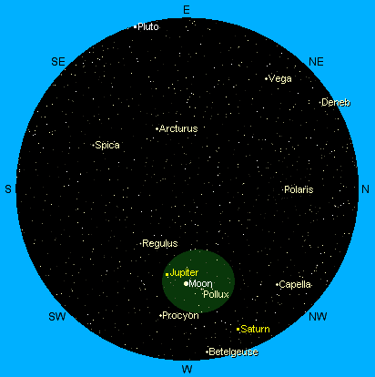 (Screenshot courtesy of the wonderful Sky View Café
applet)
(Screenshot courtesy of the wonderful Sky View Café
applet)
(Note: The three objects aren't as close together as it may look in this picture. The sky is big.) These screenshots show how it will look at 10 PM Mountain Daylight Time.
Below is a 45-degree chunk of sky looking due west. This will give you a better idea of how the sky will look as you face west. You'll probably see Pollux and Castor quite clearly. Castor is the bright star directly to the right of Pollux. Castor and Pollux will appear to make a horizontal line at this time.
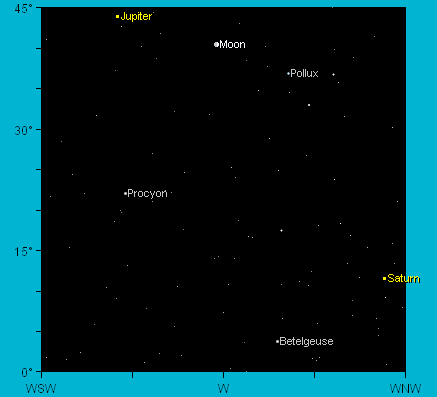
It shouldn't be hard to find. Look west. The moon will be the brightest object in the sky, and Jupiter will be the second-brightest. Follow the line from Jupiter to the moon. Pollux is by far the brightest star along that line (it has a dimmer twin Castor, which will be on the right.) The moon is in the center and Jupiter and Pollux are equal distances on either side of the moon. Follow the wise men. Bring gold. I already have lots of frankincense and myrrh.
Alan's Editorializing : This article also underlines one of the things I am growing to miss in most physical equations and all programs written in other languages... the loss of units. Everything is an unexplained number, and inscrutable conversion factors are strewn liberally throughout. This is exactly the type of thing that Frink was designed to address. For example, a line in the article indicates:
The parallax-to-distance formula is simple: d=1/p, where p is the parallax angle in arcseconds and d is the distance in parsecs (3.26 light-years).
This description is unfortunate. 1 divided by an angle (which is
dimensionless) is still dimensionless, not
a distance. This is
better specified by saying that the formula is distance=(orbital
radius)/(parallax angle). Since the parallax angles are specified with
respect to Earth's orbital radius, you can write the equation as d = au/p
. " au
" is an astronomical
unit, the average distance between the Earth and the Sun, which is included
in Frink's standard data file. Then, p can be specified in any
angular units and distance can be automatically converted to light-years or
light-days instead of parsecs (or into feet, if you want). As always, Frink makes the units of measurement transparent, and helps to ensure
that your calculations make sense.
So, using the Hipparcos
satellite's measurements for the parallax of the closest star, Proxima
Centauri (okay, second-closest, smartypants):
au / (.7723 arcsec) -> lightyears
4.223182420960891
This way, we learn something about the nature of the physical calculation which we can generalize, rather than having an equation that only works with one weird system of measurement. (Although professional astronomers like to use parsecs, I think it's a horrible, intentionally exclusive, geocentric measurement and they're just being difficult. There was even an article in Sky & Telescope a while back which intimated that some astronomers would sneer and giggle at you if you used light-years in a professional publication or speech.) Using our deeper knowledge, we can see how much more accurate the Hipparcos satellite would be if it were put into Jupiter's orbit, or how accurate its instruments need to be to achieve a certain accuracy in distance measurements. We've learned something more general.
Below is the same program as in Sky & Telescope, but more flexible. You can enter the exact second of your birth using any of the date formats that Frink recognizes. You enter the desired age as "12314 days" or "1 billion seconds" or any other duration. The program uses thefunction to calculate the target date with leap seconds accounted for . So you don't celebrate on the wrong second within the minute.
birthdate = parseDate[input["Enter your birthdate: "]]
str = input["Enter desired age: "]
age = eval[str]
println["You will be $str old on " + addLeap[birthdate,age]]
Enter your birthdate:
1969-08-19 04:54 PM Mountain
Enter desired age:
1 billion seconds
You will be 1 billion seconds old on AD 2001-04-27
06:40:15.653 PM (Fri) Mountain Daylight Time
Finding Your Own Star
Now you want your own star, don't you? You might take a look at a list of the brightest stars in the sky and look the stars' distances in light-years. This will give you an idea of the bright stars, and give you their Hipparcos catalog numbers. Using the Hipparcos catalog number given in that table, you can look up that star from this Hipparcos search form, find its Geometrical Parallax (field H11, which is probably given in milliarcseconds) and plug that number into the equation shown above. At some point, I may make a Frink Server Page that automates this. But you might learn more just by doing the calculations yourself.
Whether you have a kid who is 8.6 years old (for Sirius which is the brightest star in the sky and 3141 light-days away,) someone turning 11.4 (Procyon), turning 16.8 (Altair) or someone turning 65.1 (Aldebaran,) a star is a great gift and might just start a love of astronomy. I can't promise that the moon and the planets will line up for them , though.
Note that there is some uncertainty in measuring parallaxes, often several percent, and thus the dates are somewhat uncertain, so it's a gift you can give any time around the date. For example, the standard error for the parallax of Pollux is 0.87 milliarcseconds (parallax error is field H16 in the Hipparcos catalog, specified in milliarcseconds) which leads to an actual date that can vary from around January 17, 2003 to August 27, 2003 -- a range of over 7 months. Just have fun and celebrate your stars when you want!
Model Solar System
This one is fun. I didn't have a grasp of the size difference between the Earth and the Moon so I wanted to make a little scale model in my home. It would be best to use spheres of the appropriate sizes, but I don't have that many balls. Instead, I decided to cut circles out of paper. My deciding dimension was the size of the piece of paper I used to cut out the pieces. I could only get a 7-inch diameter circle for the Earth (3.5-inch radius), so this defined my scale, which I saved in a variable for use in later calculations:
scale = earthradius / (3.5 inches)
7.166851856017998E7
The standard data file contains information about the dimensions of the
planets, earthradius
being one of those. Now how big should
the Moon circle be?
moonradius / scale -> inches
0.9547455176283174
Okay, using my rolling ruler, I cut out a circle with radius 0.95 inches (diameter 1.9 inches). There's the Moon. It's interesting to see the difference in size between the Earth and Moon:
Now, to place them properly... how far away should they be at that scale?
moondist / scale -> feet
17.59705489913335
Okay, stick the Earth to one wall, and then measure a distance 17.5 feet away, and stick the Moon to that. Installed!
From each vantage point, you can see how big the other actually looks from that distance. Standing by the Earth, you can see how big the Moon looks (you've seen the Moon, but it's a smaller angle than you might guess... the Moon really doesn't take up much sky, only about half a degree in diameter.) You can verify this by holding a fingernail out at arm's length, comparing it to the size of your Moon model, and then going outside and doing the same to the Moon, if you can see it.
Now walk over to the Moon and look at the Earth. It would be pretty big!
Earth would appear about 3.66 times wider in diameter (in Frink notation, earthradius/moonradius
, or 13.4 times larger in area ( pi earthradius^2 / (pi moonradius^2)
).
Just to verify, I wanted to make sure that the visible angles in my model
match real life. The visual angle of an object which does not subtend a
large angle can be expressed as angle = width / distance
. The
angle normally comes out in radians if width and distance are in the same
units, but this is Frink. You can get the answer out in degrees, or
arcminutes if that's where your heart lies:
1.9 inches / (17.5 feet) -> arcminutes
31.10342316424469
Yep, that's just the right number of arcminutes. From Earth, the Sun and the Moon both appear just over half a degree in diameter, or about 32 arcminutes (an arcminute is 1/60 of a degree). It all works out. Note that in the standard data file, radians are dimensionless units (a radian is defined as "1".) This is because radians are dimensionless units, but you can convert values in radians to other angular units.
By the way, a more accurate angular formula that is valid for large and small angles subtended by a sphere with a given radius at a specified distance is:
2 arcsin[radius/(radius + distance)] -> degrees
Note that inverse trigonometric functions ( arcsin
, arccos
, arctan
) have their output in radians.
This is easily converted to whatever angular units you want, as above. You
don't see that the output is in radians (if you use the standard data file)
because radians are dimensionless numbers. You just gotta be a bit careful
here, or make the minor change in your units file to make radians a
fundamental dimension. (Read the documentation in the units file... the
units file is otherwise radians-correct.)
Nostalgic Digression: I remember a cool black-and-white movie we saw in my Kindergarten class about making a scale model of the solar system. It involved a huge vertical circular sign representing the Sun that somebody had built for the film and a car driving a measured distance away to look at it. (A bit confusing, though. I remember them saying "here we are, 93 million miles away!" and they were still in the same park.) Good stuff, and I'm glad I finally made my own model. It helps me understand how cool the Apollo missions were. But my enthusiasm is tempered by the fact that I'm just now figuring out stuff they tried to teach me in Kindergarten.
Now go make your own model. Pick your own scale to fit your surroundings and materials. It's fun. In my model, Jupiter would have to be a sphere 6.59 feet in diameter, placed about 5.5 miles away right now. I'll have to get a bigger place.
Now that you know how to calculate the size in Frink yourself, I've gone ahead and built a Frink Server Page that lets you design your own!
Homework: In your model, figure and/or plot the following:
- Orbit of the Space Shuttle (about 300 km above the surface of the Earth) Wow. That's barely up there.
- Orbit of a geosynchronous satellite (42164 km from the center of the Earth, or about 22300 miles from the surface of the Earth.) Stand this far away from the Earth circle... that's how big it would look.
- The sizes of the Sun, other planets, and their moons.
- The speed of light in your model.
Saving Hundreds of Millions of Dollars
"The MCO [Mars Climate Orbiter] MIB [Mishap Investigation Board] has determined that the root cause for the loss of the MCO spacecraft was the failure to use metric units in the coding of a ground software file, "Small Forces," used in trajectory models. Specifically, thruster performance data in English units instead of metric units was used in the software application code titled SM_FORCES (small forces)."
-- Mars Climate Orbiter Mishap Investigation Board, Phase I Report
This is not to take away from the designers of a wonderfully complex spacecraft that can travel to Mars; that's an incredibly difficult problem, and I couldn't do it. However, this is just the type of error that Frink was designed to help avoid, and because I make these type of errors a lot, I've designed this tool to help me. Frink tracks units through all calculations and makes conversions between them transparent. This is why I'm working toward making Frink a feasible solution for calculations of this type.
Update: I received the following from Peter Norvig :
"I ran across Frink, and as a member of the MCO review board, I appreciate your efforts. Note, however that more than just language support is necessary. First, you'd have to have conventions on data I/O -- the misinterpreted data was from a file, not from another function in the program. Also, there was an issue of software reuse -- the errant portion of the system had been used before on a previous mission, and in that case it was used in a non-critical, non-navigational way. It was not properly reviewed because the team did not realize that in MCO it became critical."
The points above are well-taken. Proper parsing of units can be easily achieved in Frink with a simple, appropriate comment in the data file.unittable.frink shows how Frink can parse a file containing units of measure. All that is needed is to add a single comment to the data file that contains the units of measure of each data column. Frink then reads each column with the appropriate units of measure and scale, using any units of measure that Frink knows about as input, and Frink parses them and works with them properly. See itssample data file.
Frink and its eval[x]
function could always trivially handle
the case where each number in a file has its units of measure specified
with the number, e.g. " 3.5 km/s
". That's literally zero
effort to parse with Frink, and is slightly less compact, but
that's a very small price to pay, compared to mission failure.
Of course, there's no simple solution for someone completely not reading the specification documents, but the fact that a file completely omits any units of measure would be a good warning flag to double-check your sources, I'm growing to fear and avoid any system that treats every physical measurement as an unexplained dimensionless number, as most programming languages have for the past few decades. We can do better.
Changing Syntax
Keep in mind that the syntax represented in this document will change as Frink evolves. The current parser just makes it easier for me to test certain features, and I intentionally refuse to spend a lot of time on it at this point. The internals of the language should be the first concern, and the external representation is free to change. Frink should be equally usable whether you want to load and save your data in the current mathematical notation, in a (LISP-like) prefix notation, in a (HP calculator-like) Reverse-Polish postfix notation, from a visually-based GUI, in MathML, TeX, XML, or whatever other flavor-of-the-month format the kids are crazy about these days. The internals of the language are intentionally agnostic on this point, as they should be in a flexible design.
On the other hand, I always want to keep Frink easy to use and transparent for the quick calculations as it is now. Turning it into a language that forces an encumbering programming paradigm is out of the question.
Alan's Unsolicited Advice: Anytime you're involved with a project where you hear people saying "we want to use 'X' technology" before they've even thought about representing the problem they're trying to solve, look up for the cloud of doom, which floats nigh. It's like hiring a carpenter, who, before he knows what you want to make, insists on using mortice-and-tenon joints.
Acknowledgements
OROMatcher
"This product includes software developed by the Apache Software Foundation ( http://www.apache.org/ )."
They made me say that. The included part is the Jakarta ORO regular expression library. I hacked it significantly so that it would compile and run on a Java 1.1 platform (so that Frink can be used on small devices running PersonalJava 1.1 and run in the JVM in just about any browser out there.)
ORO is included under ORO licensing terms .
Someday, I'll probably get rid of ORO altogether and use the regular expression libraries available in Java 1.4 and later, but this will require abandoning platforms currently supported by Frink (which runs on Java 1.1 and later.) Some features would be lost, though.
JavaCUP
JavaCUP is included under the following licensing terms: JavaCUP license. Note that the JavaCUP package itself is not included in Frink, but is used to generate a parser class.
JFlex
Frink's lexical analyzer is generated by JFlex . Since this was generated from Frink's own specification, Frink may use the generated code without restriction according to JFlex's licensing terms. The JFlex package itself is not included in Frink--it is only used to generate a lexer class.
Donate to Frink
If you've gotten this far, hopefully you've seen something you liked. If you find Frink useful, I'd appreciate if you took a look at some of the ways you can donate to Frink's development . Thanks!
Please send comments or questions to Alan Eliasen .
Recommend
About Joyk
Aggregate valuable and interesting links.
Joyk means Joy of geeK