Lei Mao's Website – Introduction to Bayesian Filter

Introduction

Bayesian filter is one of the fundamental approaches to estimate the distribution in a process where there are incoming measurements. It used to be widely used in localization problems in robotics. I had some experience previously in particle filter which is one of the extensions of Bayesian filter. However, when it comes to the math form of the model, I would sometimes forget. Here I am writing this article post to document the basic concept of Bayesian filter and the math related to it.

We have a stream of observation data from time step 1 to time step t:

{z1,z2,⋯,zt}

If possible, we also have a stream of action data from time step 1 to time step t:

{u1,u2,⋯,ut}

Our goal is given {z1,z2,⋯,zt} and possibly {u1,u2,⋯,ut}, we would like to estimate the distribution of robot state at time step t, i.e., calculate the probability or probability density of any possible hidden state xt. The state is hidden to the robot, and it could be discrete or continuous. For example, the state could be {ct} where ct is the coordinates of robot in the map, or {ct,pt} where pt is the pose (velocity and orientation) of robot in the map.

Statistically, we are predicting a posterior distribution called “Belief”:

Bel(xt)=P(xt|u1,z1,u2,z2,⋯,ut,zt)=P(xt|z1:t,u1:t)

It should be noted that when we predict the state of robot in Bayesian filter, we care more about the distribution of states Bel rather than the probability or probability density of certain single state Bel(xt).

Models

We have a parameterized sensor model P(z|x) which given the state xt predicts the distribution of observations at time step t.

We also have a parameterized action model P(x|u,x′) which given the state xt−1 and action ut predicts the distribution of state at time step t.

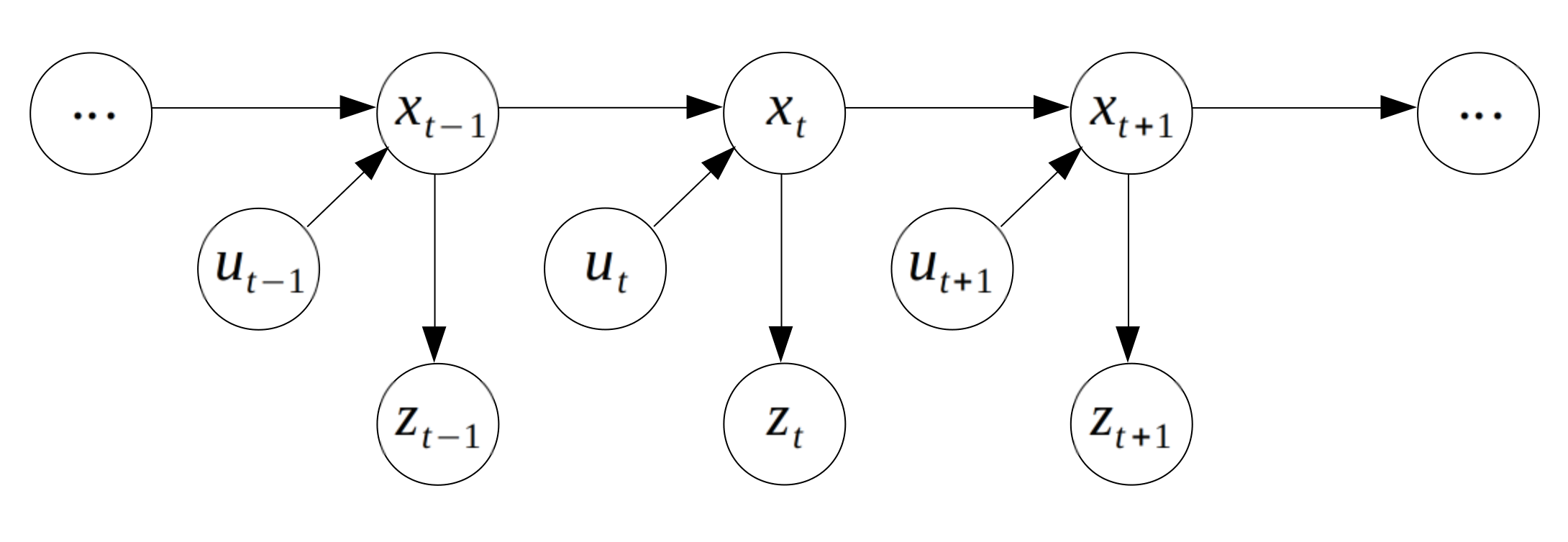
The Bayesian filter usually assumes the process is a first-order Markov chain model.

P(zt|x0:t,z1:t,u1:t)=P(zt|xt)

P(xt|x1:t−1,z1:t−1,u1:t)=P(xt|xt−1,ut)

We will use these two assumptions in our math derivations.

Graph

The whole process with assumptions could be described using a graph known as the Hidden Markov Model (HMM).

Predicted Belief

Predicted belief ¯Bel is defined as the probability distribution of state at time step t, given the observation and possibly action from time step 1 to t−1. More formally,

¯Bel(xt)=P(xt|z1:t−1,u1:t)

Using probability chain rule and property of total probability,

¯Bel(xt)=P(xt|z1:t−1,u1:t)=∫P(xt|xt−1,z1:t−1,u1:t)P(xt−1|z1:t−1,u1:t)d(xt−1)=∫P(xt|xt−1,z1:t−1,u1:t)Bel(xt−1)d(xt−1)

Note that P(xt−1|z1:t−1,u1:t)=Bel(xt−1).

We apply our Markov assumptions,

P(xt|xt−1,z1:t−1,u1:t)=P(xt|xt−1,ut)

We then get

∫P(xt|xt−1,z1:t−1,u1:t)Bel(xt−1)d(xt−1)=∫P(xt|xt−1,ut)Bel(xt−1)d(xt−1)

Therefore,

¯Bel(xt)=∫P(xt|xt−1,ut)Bel(xt−1)d(xt−1)

Note that P(xt|xt−1,ut) is calculated our action model at time step as described above.

Belief

Bel(xt)=P(xt|z1:t,u1:t)=P(xt|z1:t−1,zt,u1:t)

We apply Bayes’ theorem

Bel(xt)=P(xt|z1:t−1,zt,u1:t)=P(zt|z1:t−1,xt,u1:t)P(xt|z1:t−1,u1:t)P(zt|z1:t−1,u1:t)

We further apply our Markov assumptions,

P(zt|z1:t−1,xt,u1:t)=P(zt|xt)

So far we have,

P(xt|z1:t−1,zt,u1:t)=P(zt|xt)P(xt|z1:t−1,u1:t)P(zt|z1:t−1,u1:t)

The denominator P(zt|z1:t−1,u1:t) is a normalization term, where

P(zt|z1:t−1,u1:t)=∫P(zt|z1:t−1,xt,u1:t)P(xt|z1:t−1,u1:t)d(xt)=∫P(zt|xt)P(xt|z1:t−1,u1:t)d(xt)

We usually use a constant value to replace the denominator. So we have

Bel(xt)=ηP(zt|xt)P(xt|z1:t−1,u1:t)

We further note that ¯Bel(xt)=P(xt|z1:t−1,u1:t), therefore

Bel(xt)=ηP(zt|xt)¯Bel(xt)

Note that P(zt|xt) is calculated from the sensor model at the time step as we described above.

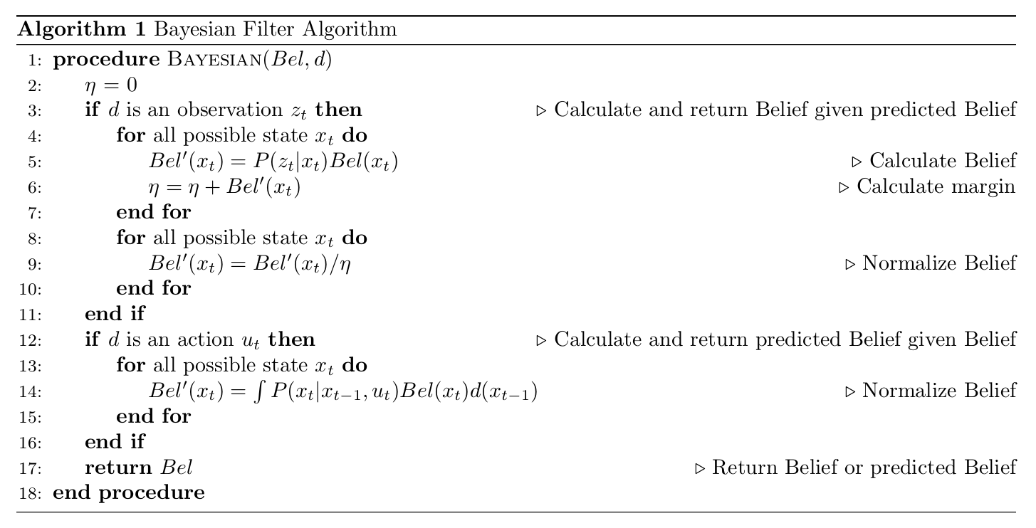
Algorithm

We are able to calculate all the three components at any time step essentially in Bayesian filter using the mathematical relationships between them we have just figured out.

• Predicted Belief ¯Bel(xt)
• Belief Bel(xt)
• Action model P(xt|xt−1,ut)
• Sensor model P(zt|xt)

Here model means some probability distribution. The parameters of the action model and sensor model are usually fixed and not going to change in Bayesian filter. Making or calibrating the action model and sensor model are often relatively easier and were done before Bayesian filter.

The filter process is basically, at each time step, we calculate the Bel(xt) and ¯Bel(xt) for each possible states using the math described above, and we update the Bel(xt) to ηP(zt|xt)¯Bel(xt) for each possible states. By doing this iteratively, the three distributions might tend to converge.

More formally, the Bayesian filter algorithm could be described as follows:

Final Remarks

The Bayesian filter algorithm above described the general process. To do it concretely, there are generally two approaches: Kalman filter and Particle filter. We may talk about these two filters in the future.

References

---

Introduction to Bayesian Filter was published on March 21, 2019 and last modified on March 21, 2019 by Lei Mao.