Log-Spherical Mapping in SDF Raymarching

Log-spherical Mapping in SDF Raymarching

Pierre Cusa <[email protected]>

February 2019 (history)

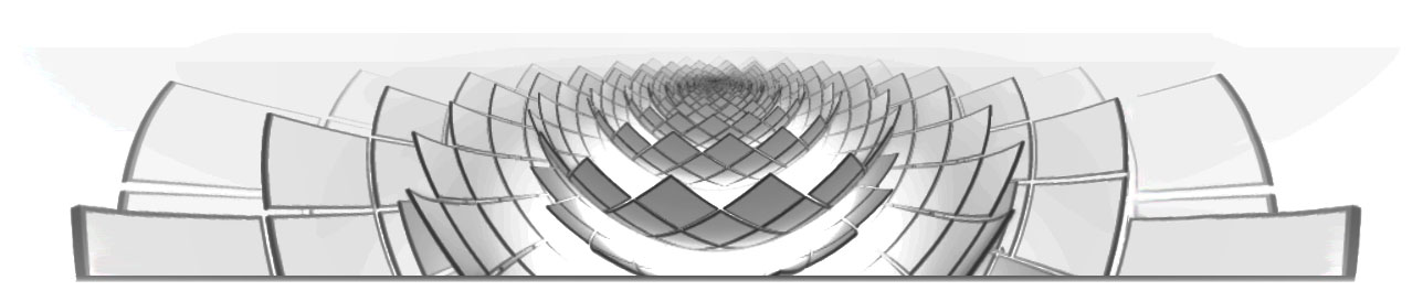
In this post, I'll describe a set of techniques for manipulating signed distance fields (SDFs) allowing the creation of self-similar geometries like the flower above. Although these types of geometries have been known and renderable for a long time, I believe the techniques described here offer much unexplored creative potential, since they allow the creation of raymarchable SDFs of self-similar geometries with an infinite level of visual recursion, which can be explored in realtime on the average current-gen graphics card. This is done by crafting distance functions based on the log-spherical mapping, which I'll explain starting with basic tilings and building up to the recursive shell transformation.

Log-polar Mapping in 2D

Conversions between log-polar coordinates $(\rho, \theta)$ and Cartesian coordinates $(x, y)$ are defined as:

$$ \tag{1} \begin{cases} \rho = \log\sqrt{x^2 + y^2}, \cr \theta = \arctan\frac{y}{x}. \end{cases} $$ $$ \tag{2} \begin{cases} x = e^\rho\cos\theta,\hphantom{\sqrt{x^2+}} \cr y = e^\rho\sin\theta. \end{cases} $$

The conversion $(2)$ can be used as an active transformation, the inverse log-polar map, in which we can consider $(\rho, \theta)$ as the Cartesian coordinates before the transformation, and $(x, y)$ after the transformation. Applying this to any geometry that regularly repeats along the $\rho$ axis results in a self-similar geometry. Let's apply it to a grid of polka dots to get an idea of how this happens.

We'll be implementing this in GLSL fragment shaders, which means everything needs to be reversed: instead of defining shapes and applying transformations to them, we first apply the inverse of those transformations to the pixel coordinates, then we define the shapes based on the transformed coordinates. This is all done in a few lines:

float logPolarPolka(vec2 pos) {
    // Apply the forward log-polar map
    pos = vec2(log(length(pos)), atan(pos.y, pos.x));

    // Scale everything so tiles will fit nicely in the ]-pi,pi] interval
    p *= 6.0/PI;

    // Convert pos to single-tile coordinates
    pos = fract(pos) - 0.5;

    // Return color depending on whether we are inside or outside a disk
    return 1.0 - smoothstep(0.3, 0.31, length(pos));
}

And here is the result in a complete shader with some extra controls:

/*
Inverse log-polar map applied to a grid polka dots.

In traditional 3D, the steps to do this would be:
1. Define the geometry for a polka dot
2. Apply a regular tiling
3. Apply the inverse log-polar map

Since this is a fragment shader, all steps are reversed and applied in reverse
order:
1. Apply the forward log-polar map to the current pixel coordinates
2. Use fract() to turn tiled coordinates into single-tile coordinates
3. Return color using the equation for a disk centered on the origin
*/

precision mediump float;
#define M_PI 3.1415926535897932384626433832795

// Inputs
varying vec2 iUV;
uniform float iTime;
uniform vec2 iRes;

// These lines are parsed by dspnote to generate sliders
uniform float rho_offset; //dspnote param: 0 - 1
uniform float theta_offset; //dspnote param: 0 - 1

float scale = 6.0/M_PI;
vec3 diskColor = vec3(0.4, 0.4, 0.3);
vec3 hBarColor = vec3(0.2, 1.0, 0.2);
vec3 vBarColor = vec3(1.0, 0.2, 0.2);

vec2 logPolar(vec2 p) {
	p = vec2(log(length(p)), atan(p.y, p.x));
	return p;
}

float line(float pos, float aaSize) {
	return smoothstep(-1.3*aaSize, -0.5*aaSize, pos) - 
		smoothstep(0.5*aaSize, 1.3*aaSize, pos);
}

float disk(vec2 pos, float aaSize) {
	return 1.0-smoothstep(0.3-aaSize, 0.3+aaSize, length(pos));
}

vec3 polka(vec2 p, float aaSize) {
	p *= scale;
	vec2 diskP = p - vec2(rho_offset, theta_offset)*3.0;
	diskP = fract(diskP) * 2.0 - 1.0;
	vec3 ret = vec3(1.0);
	ret = mix(ret, diskColor, disk(diskP, aaSize));
	ret = mix(ret, hBarColor, line(p.x, aaSize));
	ret = mix(ret, vBarColor, line(p.y, aaSize));
	return ret;
}

vec3 cartesianPolka(vec2 p) {
	p *= 4.0;
	float aaSize = length(1.0/iRes)*14.0;
	vec3 ret = polka(p, aaSize);
	if (p.y > M_PI || p.y < 0.0-M_PI)
		ret *= 0.6;
	return ret;
}

vec3 logPolarPolka(vec2 p) {
	p *= 1.5;
	float aaSize = length(logPolar(p) - logPolar(p+1.0/iRes)) * 3.5;
	return polka(logPolar(p), aaSize);
}

void main() {
	vec2 p = iUV*2.-1.;
	p.x *= iRes.x/iRes.y;
	vec2 quarter = vec2(iRes.x/iRes.y * 0.5, 0);
	vec3 ret;
	if (p.x < 0.0)
		ret = cartesianPolka(p + quarter);
	else
		ret = logPolarPolka(p - quarter);
	gl_FragColor = vec4(ret, 1.0);
}

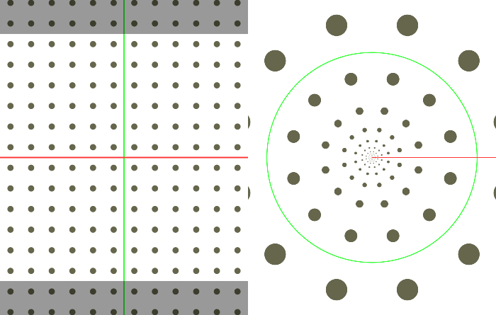
Log-polar tiling in 2D. Controls perform translation before mapping. Red axis: $\rho$, green axis: $\theta$

Note how regular tiling yields self-similarity, $\rho$-translation yields scaling, and $\theta$-translation yields rotation. Also visible, the mapping function's domain does not cover the whole space, but is limited to $\theta\in\left]-\pi, \pi\right]$ as represented by the dark boundaries.

Estimating the Distance

The above mapping function works well when applied to an implicit surface, but in order to prepare for 3D raymarching, we should apply it to a distance field, and obtain an equally correct distance field. Unfortunately, the field we obtain is heavily distorted as visualized below on the left side: the distance values are no longer correct since they are shrunk along with the surface. In order to correct for this, consider that the mapping effectively scales geometry by the radial distance $r=\sqrt{x^2 + y^2}$ (proof too large to fit in the margin). Furthermore, as Inigo Quilez notes , when scaling a distance field, we should multiply the distance value by the scaling factor. Thus the simplest correction is to multiply the distance by $r$. In most cases, this correction gives a sufficiently accurate field for raymarching.

/*
Visualization of the field distortion caused by the log-polar map.

The scene is generated following the same steps as in logpolar_polka.glsl:
1. Apply the forward log-polar map to the current pixel coordinates
2. Use fract() to turn tiled coordinates into single-tile coordinates
3. Find the distance value to a disk centered on the origin
4. Turn distance value into color using fract palette

*/

precision mediump float;
#define M_PI 3.1415926535897932384626433832795

// Inputs
varying vec2 iUV;
uniform float iTime;
uniform vec2 iRes;

// Parsed by dspnote to generate sliders
uniform float rho_offset; //dspnote param: 0 - 1

float scale = 6.0/M_PI;

vec2 logPolar(vec2 p) {
	p = vec2(log(length(p)), atan(p.y, p.x));
	return p;
}

// for visualization: smooth fract (from a comment by Shane)
float sFract(float x, float s) {
	float is = 1./s-0.99;
	x = fract(x);
	return min(x, x*(1.-x)*is)+s*0.5;
}

vec3 distanceGradient(float d, float aa) {
	vec3 ret = vec3(sFract(abs(d*3.0), aa));
	ret.x = 1. - smoothstep(-0.5*aa, 0.5*aa, d);
	ret *= exp(-1.0 * abs(d));
	return ret;
}

float disk(vec2 pos) {
	return length(pos) - 0.3;
}

float polka(vec2 p) {
	p *= scale;
	vec2 diskP = p - vec2(rho_offset, 0.0)*3.0;
	diskP = fract(diskP) * 2.0 - 1.0;
	return disk(diskP);
}

vec3 logPolarPolka(vec2 p) {
	p *= 1.5;
	vec2 lp = logPolar(p);
	float aa = length(lp - logPolar(p+1.0/iRes)) * 35.;
	if(aa>1.) aa = 1.;
	return distanceGradient(polka(lp), aa);
}

vec3 correctedPolka(vec2 p) {
	p *= 1.5;
	vec2 lp = logPolar(p);
	float aa = length(1.0/iRes) * 35.;
	return distanceGradient(polka(lp) * exp(lp.x), aa);
}

void main() {
	vec2 p = iUV*2.-1.;
	p.x *= iRes.x/iRes.y;
	vec2 quarter = vec2(iRes.x/iRes.y * 0.5, 0);
	vec3 ret;
	if (p.x < -0.01)
		ret = logPolarPolka(p + quarter);
	else if (p.x > 0.01)
		ret = correctedPolka(p - quarter);
	else
		ret = vec3(0.0);
	gl_FragColor = vec4(ret, 1.0);
}

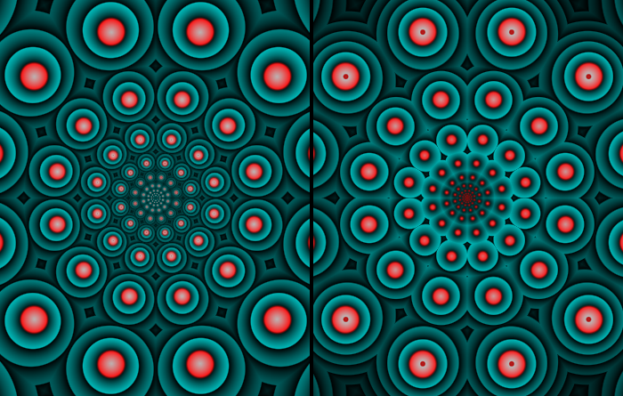
Distance field correction. Left: distorted field, right: corrected field. Colors represent the distance field's contour lines, red: negative, blue: positive.

Log-polar Mapping in 3D

The above 2D map can be simply applied in 3D space by picking two dimensions to transform. However, this means the geometry will get scaled in those two dimensions but not in the remaining dimension (in fact, geometry will be infinitely slim at the origin, and infinitely fat at the horizon). This is a problem because SDF scaling must be uniform, but we can easily correct this by scaling the remaining dimension proportionally to the others, using the same $r$ factor as before. If we're tiling spheres, this would give us the following distance function:

#define SCALE 6.0/PI

float sdf(in vec3 pos3d)
{
    // Choose 2 dimensions and apply the forward log-polar map
    vec2 pos2d = pos3d.xz;
    float r = length(pos2d);
    pos2d = vec2(log(r), atan(pos2d.y, pos2d.x));

    // Scale pos2d so tiles will fit nicely in the ]-pi,pi] interval
    pos2d *= SCALE;

    // Convert pos2d to single-tile coordinates
    pos2d = fract(pos2d) - 0.5;

    // Get ball distance;
    // Shrink Y coordinate proportionally to the other dimensions;
    // Return distance value multiplied by the final scaling factor
    float mul = r/SCALE;
    return (length(vec3(pos2d, pos3d.y/mul)) - radius) * mul;
}

Distance functions made using this technique work well with raymarching:

/*
Inverse log-polar map applied to 2 dimensions of a 3D scene.

Uses a similar process to logpolar_polka.glsl. See the `sdf` function.
*/

precision mediump float;
#define M_PI 3.1415926535897932384626433832795
#define AA 2

// Inputs
varying vec2 iUV;
uniform float iTime;
uniform vec2 iRes;

// These lines are parsed by dspnote to generate sliders
uniform float camera_y; //dspnote param: 0.5 - 3
uniform float rho_offset; //dspnote param: 0 - 10
uniform float density; //dspnote param: 5 - 50, 13
uniform float radius; //dspnote param: 0.05 - 1, 0.9

float height = 0.01;
float lpscale;

float sdf(in vec3 p3d)
{
	// Choose 2 dimensions and apply the forward log-polar map
	vec2 p = p3d.xz;
	float r = length(p);
	p = vec2(log(r), atan(p.y, p.x));

	// Scale everything so it will fit nicely in the ]-pi,pi] interval
	p *= lpscale;
	float mul = r/lpscale;

	// Apply rho-translation, which yields zooming
	p.x -= rho_offset + iTime*lpscale*0.23;
	
	// Turn tiled coordinates into single-tile coordinates
	p = mod(p, 2.0) - 1.0;

	// Get rounded cylinder distance, using the original Y coordinate shrunk
	// proportionally to the other dimensions
	return (length(vec3(p, max(0.0, p3d.y/mul))) - radius) * mul;
}

vec3 color(in vec3 p)
{
	vec3 top = vec3(0.3, 0.4, 0.5);
	vec3 ring = vec3(0.6, 0.04, 0.0);
	vec3 bottom = vec3(0.3, 0.3, 0.3);
	bottom = mix(vec3(0.0), bottom, min(1.0, -1.0/(p.y*20.0-1.0)));
	vec3 side = mix(bottom, ring, smoothstep(-height-0.001, -height, p.y));
	return mix(side, top, smoothstep(-0.01, 0.0, p.y));
}

// Adapted from http://iquilezles.org/www/articles/normalsSDF/normalsSDF.htm
vec3 calcNormal(in vec3 pos)
{
	vec2 e = vec2(1.0,-1.0)*0.5773;
	const float eps = 0.0005;
	return normalize(
		e.xyy*sdf(pos + e.xyy*eps) + 
		e.yyx*sdf(pos + e.yyx*eps) + 
		e.yxy*sdf(pos + e.yxy*eps) + 
		e.xxx*sdf(pos + e.xxx*eps)
	);
}

// Based on http://iquilezles.org/www/articles/raymarchingdf/raymarchingdf.htm
void main() {
	lpscale = floor(density)/M_PI;
	vec2 fragCoord = iUV*iRes;

	 // camera movement	
	float an = 0.04*iTime;
	vec3 ro = vec3(1.0*cos(an), camera_y, 1.0*sin(an));
	vec3 ta = vec3( 0.0, 0.0, 0.0 );
	// camera matrix
	vec3 ww = normalize(ta - ro);
	vec3 uu = normalize(cross(ww,vec3(0.0,1.0,0.0)));
	vec3 vv = normalize(cross(uu,ww));

	vec3 tot = vec3(0.0);
	
	#if AA>1
	for(int m=0; m<AA; m++)
	for(int n=0; n<AA; n++)
	{
		// pixel coordinates
		vec2 o = vec2(float(m),float(n)) / float(AA) - 0.5;
		vec2 p = (-iRes.xy + 2.0*(fragCoord+o))/iRes.y;
		#else    
		vec2 p = (-iRes.xy + 2.0*fragCoord)/iRes.y;
		#endif

		// create view ray
		vec3 rd = normalize(p.x*uu + p.y*vv + 3.5*ww); // fov

		// raymarch
		const float tmax = 10.0;
		float t = 0.0;
		for( int i=0; i<256; i++ )
		{
			vec3 pos = ro + t*rd;
			float h = sdf(pos);
			if( h<0.0001 || t>tmax ) break;
			t += h;
		}
	
		// shading/lighting	
		vec3 col = vec3(0.0);
		if( t<tmax )
		{
			vec3 pos = ro + t*rd;
			vec3 nor = calcNormal(pos);
			float dif = clamp( dot(nor,vec3(0.57703)), 0.0, 1.0 );
			float amb = 0.5 + 0.5*dot(nor,vec3(0.0,1.0,0.0));
			col = color(pos)*amb + color(pos)*dif;
		}

		// gamma        
		col = sqrt( col );
		tot += col;
	#if AA>1
	}
	tot /= float(AA*AA);
	#endif

	gl_FragColor = vec4(tot, 1.0);
}

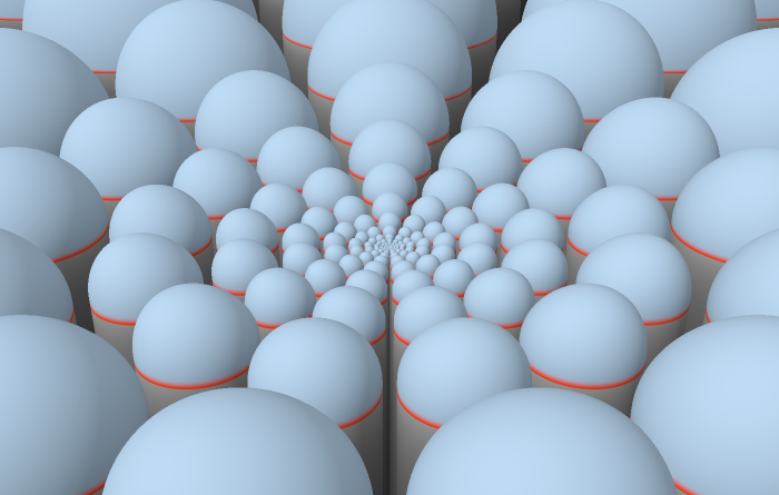
Log-polar mapping applied to two dimensions of a 3D geometry.

Log-spherical Mapping

The above technique lets us create, without loops, self-similar surfaces with an arbitrary level of detail. But the recursion still only happens in two dimensions - what if we want fully 3D self-similar geometries? Log-polar coordinate transformations can be generalized to more dimensions. Conversions between log-spherical coordinates $(\rho, \theta, \phi)$ and Cartesian coordinates $(x, y, z)$ are defined as:

$$ \tag{3} \begin{cases} \rho = \log\sqrt{x^2 + y^2 + z^2}, \cr \theta = \arccos\frac{z}{\sqrt{x^2 + y^2 + z^2}} \cr \phi = \arctan\frac{y}{x}. \end{cases} $$ $$ \tag{4} \begin{cases} x = e^\rho\sin\theta\cos\phi, \hphantom{\log x^2} \cr y = e^\rho\sin\theta\sin\phi, \cr z = e^\rho\cos\theta. \end{cases} $$

Again, conversion $(4)$ can be used as an active transformation. This is the inverse log-spherical map, which results in a self-similar geometry when applied to a regularly repeating geometry. $\rho$-translation now yields uniform scaling in all axes.

/*
Inverse log-spherical map applied to a 3D grid of cylinders.

Similar to the 2D version, let's first draft out the theoretical steps needed
to create this scene in traditional 3D:
1. Define the geometry for a cross made of two cylinders
2. Apply a regular tiling, resulting in a repeated grid of cylinders
3. Apply the inverse log-spherical map

And reverse all the steps to create a distance function:
1. Apply the forward log-spherical map to the current 3D coordinates
2. Use fract() to turn tiled coordinates into single-tile coordinates
3. Return distance using the equation for a cross of cylinders

This distance function is then used with raymarching.
*/

precision mediump float;
#define M_PI 3.1415926535897932384626433832795
#define AA 2

// Inputs
varying vec2 iUV;
uniform float iTime;
uniform vec2 iRes;

// These lines are parsed by dspnote to generate sliders
uniform float thickness; //dspnote param: 0.01 - 0.1
uniform float density; //dspnote param: 6 - 16, 8
uniform float rho_offset; //dspnote param: 0 - 10
uniform float camera_y; //dspnote param: 0.5 - 2

float shorten = 1.26;
float height = 0.01;
float lpscale;

float map(in vec3 p)
{
	// Apply the forward log-spherical map
	float r = length(p);
	p = vec3(log(r), acos(p.z / length(p)), atan(p.y, p.x));

	// Get a scaling factor to compensate for pinching at the poles
	// (there's probably a better way of doing this)
	float xshrink = 1.0/(abs(p.y-M_PI)) + 1.0/(abs(p.y)) - 1.0/M_PI;

	// Scale to fit in the ]-pi,pi] interval
	p *= lpscale;

	// Apply rho-translation, which yields zooming
	p.x -= rho_offset + iTime;
	
	// Turn tiled coordinates into single-tile coordinates
	p = fract(p*0.5) * 2.0 - 1.0;
	p.x *= xshrink;

	// Get cylinder distance
	float ret = length(p.xz) - thickness;
	ret = min(ret, length(p.xy) - thickness);

	// Compensate for all the scaling that's been applied so far
	float mul = r/lpscale/xshrink;
	return ret * mul / shorten;
}

vec3 color(in vec3 pos, in vec3 nor)
{
	return vec3(0.5, 0.5, 0.7);
}

// Adapted from http://iquilezles.org/www/articles/normalsSDF/normalsSDF.htm
vec3 calcNormal(in vec3 pos)
{
	vec2 e = vec2(1.0,-1.0)*0.5773;
	const float eps = 0.0005;
	return normalize(
		e.xyy*map(pos + e.xyy*eps) + 
		e.yyx*map(pos + e.yyx*eps) + 
		e.yxy*map(pos + e.yxy*eps) + 
		e.xxx*map(pos + e.xxx*eps)
	);
}

// Based on http://iquilezles.org/www/articles/raymarchingdf/raymarchingdf.htm
void main() {
	lpscale = floor(density)/M_PI;
	vec2 fragCoord = iUV*iRes;

	 // camera movement	
	float an = 0.1*iTime + 7.0;
	vec3 ro = vec3(1.0*cos(an), camera_y, 1.0*sin(an));
	vec3 ta = vec3( 0.0, 0.0, 0.0 );
	// camera matrix
	vec3 ww = normalize(ta - ro);
	vec3 uu = normalize(cross(ww,vec3(0.0,1.0,0.0)));
	vec3 vv = normalize(cross(uu,ww));

	vec3 bg = vec3(0.1, 0.15, 0.2)*0.3;
	vec3 tot = bg;
	
	#if AA>1
	for(int m=0; m<AA; m++)
	for(int n=0; n<AA; n++)
	{
		// pixel coordinates
		vec2 o = vec2(float(m),float(n)) / float(AA) - 0.5;
		vec2 p = (-iRes.xy + 2.0*(fragCoord+o))/iRes.y;
		#else    
		vec2 p = (-iRes.xy + 2.0*fragCoord)/iRes.y;
		#endif

		// create view ray
		vec3 rd = normalize(p.x*uu + p.y*vv + 3.5*ww); // fov

		// raymarch
		const float tmax = 3.5;
		float t = 0.0;
		for( int i=0; i<80; i++ )
		{
			vec3 pos = ro + t*rd;
			float h = map(pos);
			if( h<0.0001 || t>tmax ) break;
			t += h;
		}
	
		// shading/lighting	
		vec3 col = vec3(0.0);
		if( t<tmax )
		{
			vec3 pos = ro + t*rd;
			vec3 nor = calcNormal(pos);
			float dif = clamp( dot(nor,vec3(0.57703)), 0.0, 1.0 );
			float amb = 0.5 + 0.5*dot(nor,vec3(0.0,1.0,0.0));
			col = color(pos, nor)*amb + color(pos, nor)*dif;
		}

		// fog
		col = mix(col, bg, smoothstep(camera_y-0.2, camera_y+1.5, t));

		// gamma        
		col = sqrt( col );
		tot += col;
	#if AA>1
	}
	tot /= float(AA*AA);
	#endif

	gl_FragColor = vec4(tot, 1.0);
}

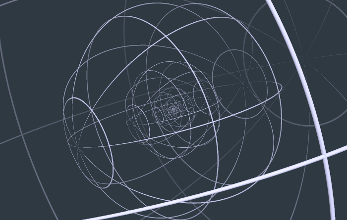
Log-spherical mapped geometry.

Similarity

With the above technique, any geometry we define will be warped into a spherical shape, with visible pinching at two poles. What if we want to create a self-similar version of any arbitrary geometry, without this deformation? For this, the mapping needs to be similar , that is, preserving angles and ratios between distances. To achieve this, we apply the forward log-spherical transformation before applying its inverse, and perform regular tiling on the intermediate geometry. The combined mapping function's domain is a spherical shell , inside which we can define any surface, and have it infinitely repeated inside and outside of itself - without relying on loops. This is implemented in the following distance function:

// pick any density and get its inverse:
float dens = 2.0;
float idens = 1.0/dens;

float sdf(in vec3 p)
{
    // Apply the forward log-spherical map
    float r = length(p);
    p = vec3(log(r), acos(p.z / r), atan(p.y, p.x));

    // find the scaling factor for the current tile
    float scale = floor(p.x*dens)*idens;

    // Turn tiled coordinates into single-tile coordinates
    p.x = mod(p.x, idens);

    // Apply the inverse log-spherical map
    float erho = exp(p.x);
    float sintheta = sin(p.y);
    p = vec3(
        erho * sintheta * cos(p.z),
        erho * sintheta * sin(p.z),
        erho * cos(p.y)
    );

    // Get distance to geometry in the prototype shell
    float ret = shell_sdf(p);

    // Correct distance value with the scaling applied
    return ret * exp(scale);
}

We can test this by putting some boxes and cylinders in the prototype shell:

/*
Log-spherical scene with preservation of shapes (similarity).

As before, let's first imagine the theoretical steps needed to create this
scene in traditional 3D:
1. Define geometry within the limits of a spherical shell, our prototile
2. Apply the forward log-spherical map, giving a deformed rectangular prototile
3. Apply a regular tiling on the prototile
4. Apply the inverse log-spherical map, bending the tiles back into shells

And reverse all the steps to create a distance function:
1. Apply the forward log-spherical map to the current 3D coordinates
2. Use fract() to turn tiled coordinates into single-tile coordinates
3. Apply the inverse log-spherical map to the coordinates
4. Return distance for a prototile

More details in sdf().
*/

precision mediump float;
#define M_PI 3.1415926535897932384626433832795
#define AA 2

// Inputs
varying vec2 iUV;
uniform float iTime;
uniform vec2 iRes;

// These lines are parsed by dspnote to generate sliders
uniform float density; //dspnote param: 1 - 5, 2
uniform float side; //dspnote param: 0.2 - 0.6, 0.5
uniform float twist; //dspnote param: 0 - 1

float shorten = 1.14;
float dens, idens, stepZoom;

// Inverse log-spherical map
vec3 ilogspherical(in vec3 p)
{
	float erho = exp(p.x);
	float sintheta = sin(p.y);
	return vec3(
		erho * sintheta * cos(p.z),
		erho * sintheta * sin(p.z),
		erho * cos(p.y)
	);
}

// Primitives from http://www.iquilezles.org/www/articles/distfunctions/distfunctions.htm
float sdBox( vec3 p, vec3 b )
{
	vec3 d = abs(p) - b;
	return min(max(d.x,max(d.y,d.z)),0.0) + length(max(d,0.0));
}

float sdCappedCylinder( vec3 p, vec2 h )
{
	vec2 d = abs(vec2(length(p.xz),p.y)) - h;
	return min(max(d.x,d.y),0.0) + length(max(d,0.0));
}

float sdCone( vec3 p, vec2 c )
{
	// c must be normalized
	float q = length(p.xz);
	return dot(c,vec2(q,p.y));
}

// Axis rotation taken from tdhooper
void pR(inout vec2 p, float a) {
	p = cos(a)*p + sin(a)*vec2(p.y, -p.x);
}

// Object placement depends on the density and is lazily hardcoded.
// Objects should be inside the spherical shell reference tile
// (ie. between its inner and outer spheres)
vec2 hiddenConeBottom = normalize(vec2(1.0, 0.55));
vec2 hiddenConeSides;
vec3 floorPos = vec3(0.0, 1.125, 0.0);

float layer(in vec3 p, in float twost)
{
	float ret = sdCappedCylinder(p+floorPos, vec2(0.6, 0.03));
	pR(p.yz, twost);
	p.x = abs(p.x) - 1.25;
	ret = min(ret, sdBox(p, vec3(side)));
	ret = max(-sdBox(p, vec3(side*2.0, side*0.9, side*0.9 )), ret);
	return ret;
}

float sdf(in vec3 pin)
{
	// Apply the forward log-spherical map (shell tiles -> box tiles)
	float r = length(pin);
	vec3 p = vec3(log(r), acos(pin.z / length(pin)), atan(pin.y, pin.x));

	// Apply rho-translation, which yields zooming
	p.x -= iTime*0.2;

	// find the scaling factor for the current tile
	float xstep = floor(p.x*dens) + (iTime*0.2)*dens;
	
	// Turn tiled coordinates into single-tile coordinates
	p.x = mod(p.x, idens);

	// Apply inverse log-spherical map (box tile -> shell tile)
	p = ilogspherical(p);
	
	// Get distance to geometry in this and adjacent shells
	float ret = layer(p, xstep*twist);
	ret = min(ret, layer(p/stepZoom, (xstep+1.0)*twist)*stepZoom);

	// Compensate for scaling applied so far
	ret = ret * exp(xstep*idens) / shorten;
	
	// Compensate for discontinuities in the field by adding some hidden
	// geometry to bring rays into the right shells
	float co = sdCone(pin, hiddenConeBottom);
	if (co < 0.015) co = ret;
	ret = min(ret, co);
	pin.x = -abs(pin.x);
	co = sdCone(pin.yxz, hiddenConeSides);
	if (co < 0.015) co = ret;
	ret = min(ret, co);

	return ret;
}

vec3 step2color(in float s)
{
	return vec3(
		abs(sin(s*23.0))*0.3, 
		abs(sin(s*13.0+7.0))*0.3, 
		abs(sin(s*19.0+5.0))*0.03
	);
}

vec3 color(in vec3 p)
{
	// If shell contents don't overlap, 
	// we can color per-shell by simply checking the rho value
	/*
	float rho = log(length(p)) - iTime*0.2;
	rho = floor(rho*dens);
	return vec3(
		abs(sin(x*23.0))*0.3, 
		abs(sin(x*13.0+7.0))*0.3, 
		abs(sin(x*19.0+5.0))*0.03
	);
	*/

	// If shell contents do overlap, we need to repeat a lot of sdf() ops
	float r = length(p);
	p = vec3(log(r), acos(p.z / r), atan(p.y, p.x));
	p.x -= iTime*0.2;
	float ofs = (iTime*0.2)*dens;
	float xstep = floor(p.x*dens) + ofs;
	p.x = fract(p.x*dens)*idens;
	p = ilogspherical(p);
	float sdf = layer(p, xstep*twist);
	if (sdf < 0.03) return step2color(xstep-ofs);
	sdf = min(sdf, layer(p/stepZoom, (xstep+1.0)*twist)*stepZoom);
	if (sdf < 0.03) return step2color(xstep+1.0-ofs);
	return vec3(0.);
}

// Adapted from http://iquilezles.org/www/articles/normalsSDF/normalsSDF.htm
vec3 calcNormal(in vec3 pos)
{
	vec2 e = vec2(1.0,-1.0)*0.5773;
	const float eps = 0.0005;
	return normalize(
		e.xyy*sdf(pos + e.xyy*eps) + 
		e.yyx*sdf(pos + e.yyx*eps) + 
		e.yxy*sdf(pos + e.yxy*eps) + 
		e.xxx*sdf(pos + e.xxx*eps)
	);
}

// Based on http://iquilezles.org/www/articles/raymarchingdf/raymarchingdf.htm
void main() {

	// inverse density, and the resulting zoom between each recursion level
	dens = density;
	idens = 1.0/dens;
	stepZoom = exp(idens);
	hiddenConeSides = normalize(vec2(1.0, side * 1.3));

	vec2 fragCoord = iUV*iRes;

	 // camera movement	
	float an = 0.1*iTime + 7.0;
	float cy = 1.+sin(an*2.+1.6)*0.8;
	vec3 ro = vec3(1.0*cos(an), cy, 1.0*sin(an));
	vec3 ta = vec3( 0.0, 0.0, 0.0 );
	// camera matrix
	vec3 ww = normalize(ta - ro);
	vec3 uu = normalize(cross(ww,vec3(0.0,1.0,0.0)));
	vec3 vv = normalize(cross(uu,ww));

	vec3 bg = vec3(0.48, 0.48, 0.8);
	vec3 tot = bg;
	
	#if AA>1
	for(int m=0; m<AA; m++)
	for(int n=0; n<AA; n++)
	{
		// pixel coordinates
		vec2 o = vec2(float(m),float(n)) / float(AA) - 0.5;
		vec2 p = (-iRes.xy + 2.0*(fragCoord+o))/iRes.y;
		#else    
		vec2 p = (-iRes.xy + 2.0*fragCoord)/iRes.y;
		#endif

		// create view ray
		vec3 rd = normalize(p.x*uu + p.y*vv + 3.5*ww); // fov

		// raymarch
		const float tmax = 3.5;
		float t = 0.0;
		for( int i=0; i<60; i++ )
		{
			vec3 pos = ro + t*rd;
			float h = sdf(pos);
			if( h<0.0001 || t>tmax ) break;
			t += h;
		}
	
		// shading/lighting	
		vec3 col = vec3(0.0);
		if( t<tmax )
		{
			vec3 pos = ro + t*rd;
			vec3 nor = calcNormal(pos);
			float dif = clamp( dot(nor,vec3(0.57703)), 0.0, 1.0 );
			float amb = 0.5 + 0.5*dot(nor,vec3(0.0,1.0,0.0));
			col = color(pos)*amb + color(pos)*dif;
		}

		// fog
		col = mix(col, bg, smoothstep(0.55+cy, 1.5+cy, t));

		// gamma        
		col = sqrt( col );
		tot += col;
	#if AA>1
	}
	tot /= float(AA*AA);
	#endif

	gl_FragColor = vec4(tot, 1.0);
}

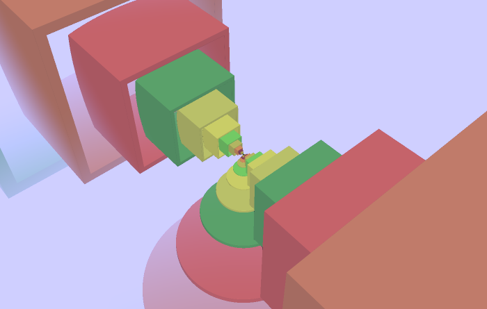
Similar log-spherical mapped geometry.

Implementation Challenges

Anyone experimenting with these techniques will inevitably run into problems due to distance field discontinuities, so it would be really scummy not to include a section on this topic. The symptoms will appear as visible holes when raymarching, as rays will sometimes overshoot the desired surface. To better understand the problem, the classic SDF debugging technique is to take a cross-section of a raymarched scene and to color it according to its distance value.

/*
Visualization of sdf discontinuities under the recursive shell tiling.
*/

precision mediump float;
#define M_PI 3.1415926535897932384626433832795
#define AA 2

// Inputs
varying vec2 iUV;
uniform float iTime;
uniform vec2 iRes;

// These lines are parsed by dspnote to generate sliders
uniform float twist; //dspnote param: 0 - 1.57

float shorten = 1.14;

// Inverse log-spherical map
vec3 ilogspherical(in vec3 p)
{
	float r = exp(p.x);
	float sintheta = sin(p.y);
	return vec3(
		r * sintheta * cos(p.z),
		r * sintheta * sin(p.z),
		r * cos(p.y)
	);
}

// Primitives from http://www.iquilezles.org/www/articles/distfunctions/distfunctions.htm
float sdBox( vec3 p, vec3 b )
{
	vec3 d = abs(p) - b;
	return min(max(d.x,max(d.y,d.z)),0.0) + length(max(d,0.0));
}

// Axis rotation taken from tdhooper
void pR(inout vec2 p, float a) {
	p = cos(a)*p + sin(a)*vec2(p.y, -p.x);
}

// density, its inverse, and the resulting zoom between each recursion level
float dens = 2.0;
float idens;
float stepZoom;

float layer(in vec3 p, in float twost)
{
	pR(p.xy, -twost);
	p.x = abs(p.x) - 1.25;
	float ret = sdBox(p, vec3(0.1));
	return ret;
}

float sdfScene(in vec3 pin)
{
	// Apply the forward log-spherical map (shell tiles -> box tiles)
	float r = length(pin);
	vec3 p = vec3(log(r), acos(pin.z / length(pin)), atan(pin.y, pin.x));

	// Apply rho-translation, which yields zooming
	p.x -= iTime*0.2;

	// find the scaling factor for the current tile
	float xstep = floor(p.x*dens) + (iTime*0.2)*dens;
	
	// Turn tiled coordinates into single-tile coordinates
	p.x = fract(p.x*dens)*idens;

	// Apply inverse log-spherical map (box tile -> shell tile)
	p = ilogspherical(p);
	
	// Get distance to geometry in this and adjacent shells
	float ret = layer(p, xstep*twist);
	ret = min(ret, layer(p/stepZoom, (xstep+1.0)*twist)*stepZoom);

	// Compensate for scaling applied so far
	ret = ret * exp(xstep*0.5) / shorten;
	return ret;
}

float sdf(in vec3 p)
{
	float ret = sdfScene(p);
	ret = min(ret, p.z);
	return ret;
}

// Adapted from http://iquilezles.org/www/articles/normalsSDF/normalsSDF.htm
vec3 calcNormal(in vec3 pos)
{
	vec2 e = vec2(1.0,-1.0)*0.5773;
	const float eps = 0.0005;
	return normalize(
		e.xyy*sdf(pos + e.xyy*eps) + 
		e.yyx*sdf(pos + e.yyx*eps) + 
		e.yxy*sdf(pos + e.yxy*eps) + 
		e.xxx*sdf(pos + e.xxx*eps)
	);
}

float aaFract(float x, float aa) { // aa: 0-1
	x = fract(x+aa*0.9);
	x += 1.0 - smoothstep(0.0, aa, x) - aa*0.5;
	return x;
}

vec3 distanceGradient(float d, float aa) {
	vec3 ret = vec3(aaFract(abs(d*3.0), aa));
	ret.x = 1. - smoothstep(-0.5*aa, 0.5*aa, d);
	ret *= exp(-1.0 * abs(d));
	return ret;
}

vec3 color(in vec3 p, in vec3 nor)
{
	if (abs(p.z)<0.0005)
		return distanceGradient(sdfScene(p)*12., 0.01);
	// Shell contents don't overlap, so we can color per-shell simply by
	// checking the rho value
	float rho = log(length(p)) - iTime*0.2;
	rho = floor(rho*dens);
	return vec3(
		abs(sin(rho*23.0))*0.3, 
		abs(sin(rho*13.0+7.0))*0.3, 
		abs(sin(rho*19.0+5.0))*0.03
	);
}

// Based on http://iquilezles.org/www/articles/raymarchingdf/raymarchingdf.htm
void main() {
	idens = 1.0/dens;
	stepZoom = exp(idens);
	vec2 fragCoord = iUV*iRes;

	 // camera movement	
	float an = 0.1*iTime + 7.0;
	vec3 ro = vec3(1.0*cos(an), 0.5, 1.0*sin(an));
	vec3 ta = vec3( 0.0, 0.0, 0.0 );
	// camera matrix
	vec3 ww = normalize(ta - ro);
	vec3 uu = normalize(cross(ww,vec3(0.0,1.0,0.0)));
	vec3 vv = normalize(cross(uu,ww));

	vec3 bg = vec3(0.48, 0.48, 0.8);
	vec3 tot = bg;
	
	#if AA>1
	for(int m=0; m<AA; m++)
	for(int n=0; n<AA; n++)
	{
		// pixel coordinates
		vec2 o = vec2(float(m),float(n)) / float(AA) - 0.5;
		vec2 p = (-iRes.xy + 2.0*(fragCoord+o))/iRes.y;
		#else    
		vec2 p = (-iRes.xy + 2.0*fragCoord)/iRes.y;
		#endif

		// create view ray
		vec3 rd = normalize(p.x*uu + p.y*vv + 3.5*ww); // fov

		// raymarch
		const float tmax = 3.5;
		float t = 0.0;
		for( int i=0; i<60; i++ )
		{
			vec3 pos = ro + t*rd;
			float h = sdf(pos);
			if( h<0.0001 || t>tmax ) break;
			t += h;
		}
	
		// shading/lighting	
		vec3 col = vec3(0.0);
		if( t<tmax )
		{
			vec3 pos = ro + t*rd;
			vec3 nor = calcNormal(pos);
			float dif = clamp( dot(nor,vec3(0.57703)), 0.0, 1.0 );
			float amb = 0.5 + 0.5*dot(nor,vec3(0.0,1.0,0.0));
			col = color(pos, nor)*amb + color(pos, nor)*dif;
		}

		// fog
		col = mix(col, bg, smoothstep(20.0, 30.0, t));

		// gamma        
		col = sqrt( col );
		tot += col;
	#if AA>1
	}
	tot /= float(AA*AA);
	#endif

	gl_FragColor = vec4(tot, 1.0);
}

Log-spherical scene with distance gradient shown in a cross-section.

Under the log-spherical mapping, repeated tiles become spherical shells contained inside of each other. Visualized above is the discontinuity in the distance gradient at the edges between shells, due to each tile only providing the distance to the geometry inside of it. Here, the "twist" parameter modifies the scene in a way that accentuates the discontinuities. This type of problem can be fixed in several ways, all of which are tradeoffs against rendering performance:

• Add hidden geometry to bring rays into the correct tile. In some cases, we know that the final geometry will approximately conform to a certain plane or other simple shape. We can estimate this shape's distance, cut off its field below a certain threshold so it's never actually hit, and combine it into the scene.
• Combine the SDF for adjacent tiles into each tile, so that the distance value takes into account more surrounding geometry. This is especially useful when the contents of each tile are close to, or touching each other.
• Shorten the raymarching steps. This can be done globally, or only locally in problematic regions.

Examples

/*
Log-spherical tiled petals. The log-spherical mapping turns slab tiles repeated
along the rho axis into concentric spherical shells.
*/

precision mediump float;
#define M_PI 3.1415926535897932384626433832795
#define AA 2

// Inputs
varying vec2 iUV;
uniform float iTime;
uniform vec2 iRes;

// These lines are parsed by dspnote to generate sliders
uniform float density; //dspnote param: 3 - 35, 26
uniform float height; //dspnote param: -0.8 - 0.8, 0
uniform float fov; //dspnote param: 0.5 - 3, 1.5
uniform float camera_y; //dspnote param: 0.4 - 2

// 25 // 8.5 // 0.5 // 1.83

float camera_ty = -0.17;
float interpos = -0.5;
float shorten = 1.;
float line_width = 0.017;
float rot_XY = 0.;
float rot_YZ = 0.785;
float radius = 0.05;
float rho_offset = 0.;
float vcut;
float lpscale;

float sdCone( vec3 p, vec2 c )
{
	// c must be normalized
	float q = length(p.xz);
	return dot(c,vec2(q,p.y));
}

void pR(inout vec2 p, float a) {
	p = cos(a)*p + sin(a)*vec2(p.y, -p.x);
}

void tile(in vec3 p, out vec3 sp, out vec3 tp, out vec3 rp, out float mul)
{
	float r = length(p);
	p = vec3(log(r), acos(p.y / length(p)), atan(p.z, p.x));
	float xshrink = 1.0/(abs(p.y-M_PI)) + 1.0/(abs(p.y)) - 1.0/M_PI;
	p.y += height;
	p.z += p.x * 0.3;
	mul = r/lpscale/xshrink;
	p *= lpscale;
	sp = p;
	p.x -= rho_offset + iTime*0.5;
	p = fract(p*0.5) * 2.0 - 1.0;
	p.x *= xshrink;
	tp = p;
	pR(p.xy, rot_XY);
	pR(p.yz, rot_YZ);
	rp = p;
}

float sdf(in vec3 p)
{
	vec3 sp, tp, rp;
	float mul;
	tile(p, sp, tp, rp, mul);
	
	// surface:
	float spheres = abs(rp.x) - 0.012;
	float leaves = max(spheres, max(-rp.y, rp.z));
	leaves = max(leaves, vcut-sp.y);
	spheres = max(spheres, vcut-sp.y+1.07);
	float ret = min(leaves, spheres);

	// intercals:
	vec3 pi = rp;
	pi.x += interpos;
	float interS = abs(pi.x) - 0.02;
	float interL = max(interS, max(-rp.y, rp.z));
	interL = max(interL, vcut-sp.y+2.);
	interS = max(interS, vcut-sp.y+3.);
	ret = min(ret, min(interL, interS));

	// 3d outline:
	// float ol = length(rp.xz) - radius*0.8;
	// ol = min(ol, length(rp.xy) - radius*0.8);
	// ol = max(ol, vcut-sp.y);
	// 2d outline:
	float ol = abs(rp.y) - radius*0.8;
	ol = min(ol, abs(rp.z) - radius*0.8);
	// cut out
	ret = max(ret, -ol);


	return ret * mul / shorten;
}

vec3 colr(in vec3 p)
{
	vec3 sp, tp, rp, ret;
	float mul;
	tile(p, sp, tp, rp, mul);

	// 2d outline
	float ol = abs(rp.y) - radius;
	ol = min(ol, abs(rp.z) - radius);

	// intercals
	vec3 pi = rp;
	pi.x += interpos;
	float inter = abs(pi.x) - 0.02;
	inter = max(inter, vcut-sp.y+2.);

	float dark = smoothstep(density*0.25, density*0.5, density - sp.y);
	dark *= dark;
	
	if (ol < line_width)
		ret = vec3 (0.6, 0.6, 0.8)*dark;
	else if (inter < 0.02)
		ret = vec3 (0.1, 0.35, 0.05)*dark;
	else
		ret = vec3 (0.1, 0.15, 0.25)*dark;
	return ret;
}

// Adapted from http://iquilezles.org/www/articles/normalsSDF/normalsSDF.htm
vec3 calcNormal(in vec3 pos)
{
	vec2 e = vec2(1.0,-1.0)*0.5773;
	const float eps = 0.0005;
	return normalize(
		e.xyy*sdf(pos + e.xyy*eps) + 
		e.yyx*sdf(pos + e.yyx*eps) + 
		e.yxy*sdf(pos + e.yxy*eps) + 
		e.xxx*sdf(pos + e.xxx*eps)
	);
}

// From http://www.iquilezles.org/www/articles/functions/functions.htm
float gain(float x, float k) 
{
	float a = 0.5*pow(2.0*((x<0.5)?x:1.0-x), k);
	return (x<0.5)?a:1.0-a;
}

vec3 gain(vec3 v, float k)
{
	return vec3(gain(v.x, k), gain(v.y, k), gain(v.z, k));
}

// Based on http://iquilezles.org/www/articles/raymarchingdf/raymarchingdf.htm
void main() {
	vcut = floor(density*0.25)*2.+0.9;
	lpscale = floor(density)/M_PI;
	vec2 fragCoord = iUV*iRes;

	 // camera movement	
	float an = 0.002*iTime + 7.0;
	vec3 ro = vec3(1.0*cos(an), camera_y, 1.0*sin(an));
	vec3 ta = vec3( 0.0, camera_ty, 0.0 );
	// camera matrix
	vec3 ww = normalize(ta - ro);
	vec3 uu = normalize(cross(ww,vec3(0.0,1.0,0.0)));
	vec3 vv = normalize(cross(uu,ww));

	vec3 bg = vec3(0.06, 0.08, 0.11)*0.3;
	bg *= 1.-smoothstep(0.1, 2., length(iUV*2.-1.));
	vec3 tot = bg;
	
	#if AA>1
	for(int m=0; m<AA; m++)
	for(int n=0; n<AA; n++)
	{
		// pixel coordinates
		vec2 o = vec2(float(m),float(n)) / float(AA) - 0.5;
		vec2 p = (-iRes.xy + 2.0*(fragCoord+o))/iRes.y;
		#else    
		vec2 p = (-iRes.xy + 2.0*fragCoord)/iRes.y;
		#endif

		// create view ray
		vec3 rd = normalize(p.x*uu + p.y*vv + fov*ww);

		// raymarch
		const float tmax = 3.5;
		float t = 0.0;
		vec3 pos;
		int iout;
		for( int i=0; i<64; i++ )
		{
			pos = ro + t*rd;
			float h = sdf(pos);
			if( h<0.0001 || t>tmax ) break;
			t += h;
			iout = i;
		}
		float fSteps = float(iout) / 64.;
	
		// shading/lighting	
		vec3 col = vec3(0.0);
		if( t<tmax )
		{
			vec3 nor = calcNormal(pos);
			float dif = clamp( dot(nor,vec3(0.57703)), 0.0, 1.0 );
			float amb = 0.5 + 0.5*dot(nor,vec3(0.0,1.0,0.0));
			col = colr(pos)*amb + colr(pos)*dif;
		}

		// glow
		float gloamt = smoothstep(0.04, 0.5, length(pos));
		float gain_pre = 1. - gloamt*0.6;
		float gain_k = 1.5 + gloamt*2.5;
		col += gain(fSteps*vec3(0.7, 0.8, 0.9)*gain_pre, gain_k);

		// fog
		col = mix(col, bg, smoothstep(0.2+camera_y, 1.6+camera_y, t));

		// gamma        
		col = sqrt( col );
		tot += col;
	#if AA>1
	}
	tot /= float(AA*AA);
	#endif

	gl_FragColor = vec4(tot, 1.0);
}

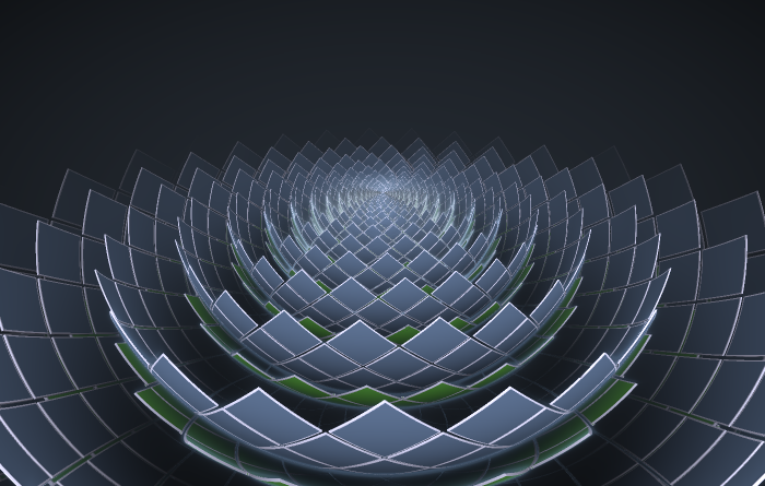
Recursive Lotus

/*
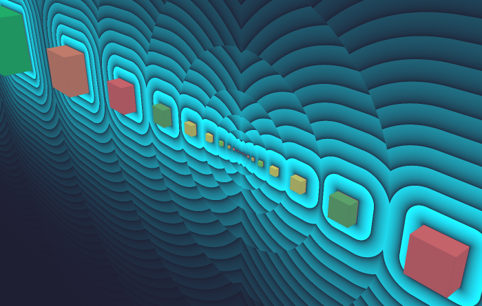
Log-polar tiled cubes. The log-polar mapping is applied to the xz coordinates of
the 3D SDF. The remaining dimension is shrunk by a factor of length(xz). In this
way, the mapping becomes uniform and the SDF distortion is greatly reduced.
*/

precision mediump float;

// Inputs
varying vec2 iUV;
uniform float iTime;
uniform vec2 iRes;

#define AA 2
#define HEIGHT 0.25
#define M_PI 3.1415926535897932384626433832795
#define LONGSTEP (M_PI*4.)

float gTime;

/* 
The tiling switches between 3 different densities at regular time points. These
switches are not instant, but propagate like a shockwave from the origin. So at
any given time during the transitions, there are two different densities, and a
boundary position between the two. These are stored in globals, set in main()
and consumed in the sdf: 
*/
float gABPos;
float gDensA;
float gDensB;

// Modified rom http://www.iquilezles.org/www/articles/distfunctions/distfunctions.htm
float sdCube( vec3 p, float b )
{
	vec3 d = abs(p) - b;
	return min(max(d.x,max(d.y,d.z)),0.0) + length(max(d,0.0));
}

// Axis rotation taken from tdhooper. R(p.xz, a) rotates "x towards z".
void pR(inout vec2 p, float a) {
	p = cos(a)*p + sin(a)*vec2(p.y, -p.x);
}

// spiked surface distance (h >= 0)
float sdSpike2D(vec2 p, float h)
{
	float d = p.y - (h*0.1)/(abs(p.x)+0.1);
	d = min(d, length(p - vec2(0, min(h, p.y))));
	float d2 = abs(p.x) - ((h*0.1)-0.1*p.y)/p.y;
	if (p.y<h && d>0.0)
		d = min(d, d2);
	return d;
}

/*
Tile space in a spiked log-polar grid.

- in `pin`: point with length(pin.xz) precomputed in pin.w
- out `density`: density of tiling
- out `cubsz`: size of cube
- returns: tiled point coordinates
*/
vec3 tile(in vec4 pin, out float density, out float cubsz)
{
	float r = pin.w;
	// switch densities in shockwaves
	density = mix(gDensA, gDensB, smoothstep(0., 0.1, r-gABPos));
	// log-polar transformation in xz; spike and proportional shrink in y
	vec3 p = vec3(
		log(r), 
		(pin.y-HEIGHT*0.1/(r+0.1))/r, 
		atan(pin.z, pin.x)
	);
	// scaling in the log-polar domain creates density
	p *= density;
	// rho-translation causes zooming
	p.x -= gTime*2.0;
	// make it a spiral by rotating the tiled plane
	pR(p.xz, 0.6435); // atan(3/4)
	// convert to single-tile coordinates
	p.xz = fract(p.xz*0.5) * 2.0 - 1.0;
	// scale and rotate the individual cubes
	// using an oscillation that spreads from the center over time
	float osc = sin(sqrt(r)-gTime*0.25-1.0);
	float cubrot = smoothstep(0.5, 0.8, osc);
	cubsz = sin(p.x*0.1)*0.29 + 0.5;
	cubsz = mix(cubsz, 0.96, smoothstep(0.7, 1.0, abs(osc)));
	pR(p.xy, cubrot);
	return p;
}

float sdf(in vec3 pin)
{
	// tile the coordinates and get cube distance
	float r = length(pin.xz);
	float cubsz, density; // out
	vec3 tiled = tile(vec4(pin, r), density, cubsz);
	float ret = sdCube(tiled, cubsz);
	// adjust the distance based on how much scaling occured
	ret *= r/density;

	// avoid overstepping:
	// add hidden surface to bring rays into the right tiles
	float pkofs = r * cubsz / density;
	float pk = sdSpike2D(vec2(r, pin.y), HEIGHT) - pkofs;
	if (pk < 0.002) pk = ret;
	ret = min(ret, pk);
	// shorten steps near the peak
	float shorten = length(pin - vec3(0., 0.25, 0.));
	shorten = 1. + 1.5*(1.-smoothstep(0., 0.22, shorten));
	ret /= shorten;

	return ret;
}

// Color the faces of cubes, reusing the tiling function.
vec3 colr(in vec3 pin)
{
	float a = 0.26;
	float b = 0.65;
	float z = 0.19;
	float cubsz, density; // out
	vec3 p = tile(vec4(pin, length(pin.xz)), density, cubsz);
	if (p.x > abs(p.y) && p.x > abs(p.z)) return vec3(z,a,b);
	if (p.x < -abs(p.y) && p.x < -abs(p.z)) return vec3(z,b,a)*0.7;
	if (p.z > abs(p.x) && p.z > abs(p.y)) return vec3(z,a,a);
	if (p.z < -abs(p.x) && p.z < -abs(p.y)) return vec3(b*0.5,z,a);
	return vec3(b,b,a);
}

// Adapted from http://iquilezles.org/www/articles/normalsSDF/normalsSDF.htm
vec3 calcNormal(in vec3 pos)
{
	vec2 e = vec2(1.0,-1.0)*0.5773;
	const float eps = 0.0005;
	return normalize(
		e.xyy*sdf(pos + e.xyy*eps) + 
		e.yyx*sdf(pos + e.yyx*eps) + 
		e.yxy*sdf(pos + e.yxy*eps) + 
		e.xxx*sdf(pos + e.xxx*eps)
	);
}

float time2density(float x)
{
	float fullMod = fract(x/(LONGSTEP*3.))*3.;
	if (fullMod > 2.) return 45.;
	else if (fullMod > 1.) return 25.;
	else return 15.;
}

// Based on http://iquilezles.org/www/articles/raymarchingdf/raymarchingdf.htm
void main() {
	// automate the shockwave transitions between densities
	gTime = iTime+1.8;
	float ltime = gTime + M_PI*6.3;
	gABPos = smoothstep(0.45, 0.6, fract(ltime/LONGSTEP))*2.2-0.2;
	gDensA = floor(time2density(ltime))/M_PI;
	gDensB = floor(time2density(ltime-LONGSTEP))/M_PI;

	vec2 fragCoord = iUV*iRes;

	 // camera movement	
	float camera_y = pow(sin(gTime*0.2), 3.)*0.2+0.7;
	vec3 ro = vec3(0., camera_y, 1.);
	vec3 ta = vec3(0.0, 0.0, 0.0);
	// camera matrix
	vec3 ww = normalize(ta - ro);
	vec3 uu = normalize(cross(ww,vec3(0.0,1.0,0.0)));
	vec3 vv = normalize(cross(uu,ww));

	vec3 tot = vec3(0.0);
	
	#if AA>1
	for(int m=0; m<AA; m++)
	for(int n=0; n<AA; n++)
	{
		// pixel coordinates
		vec2 o = vec2(float(m),float(n)) / float(AA) - 0.5;
		vec2 p = (-iRes.xy + 2.0*(fragCoord+o))/iRes.y;
		#else    
		vec2 p = (-iRes.xy + 2.0*fragCoord)/iRes.y;
		#endif

		// create view ray
		vec3 rd = normalize(p.x*uu + p.y*vv + 3.5*ww); // fov

		// raymarch
		const float tmax = 3.0;
		float t = 0.0;
		for(int i=0; i<256; i++)
		{
			vec3 pos = ro + t*rd;
			float h = sdf(pos);
			if( h<0.0001 || t>tmax ) break;
			t += h;
		}
	
		// shading/lighting	
		vec3 bg = vec3(0.1, 0.15, 0.2)*0.3;
		vec3 col = bg;
		if(t<tmax)
		{
			vec3 pos = ro + t*rd;
			vec3 nor = calcNormal(pos);
			float dif = clamp( dot(nor,vec3(0.57703)), 0.0, 1.0 );
			float amb = 0.5 + 0.5*dot(nor,vec3(0.0,1.0,0.0));
			col = colr(pos)*amb + colr(pos)*dif;
		}
		// fog
		col = mix(col, bg, smoothstep(2., 3., t));

		// gamma        
		col = sqrt(col);
		tot += col;
	#if AA>1
	}
	tot /= float(AA*AA);
	#endif

	gl_FragColor = vec4(tot, 1.0);
}

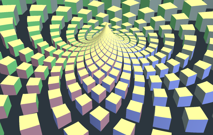
Cube Singularity

Prior Art, References and More

While I haven't found any previous utilization of the log-spherical transformation in shaders, there are many related and similar techniques that have been creatively used:

• The 2D log-polar transformation, and its related logarithmic spirals, have been used since the early days of fragment shader programming. They have also been developed into much more interesting and complex structures and related transformations. A nice example: Flexi's Bipolar Complex .
• Applying the 2D log-polar transform to 3D SDFs has been done previously, but apparently only as a cursory exploration, see knighty's Spiral tiling shader.
• Self-similar structures and zoomers have also been implemented in shaders using loops, as opposed to the loopless techniques described here. Looping strongly limits the number of visible levels of recursion for realtime, however, it allows more freedom in geometry placement while giving an exact distance. Some examples of this: Gimbal Harmonics ; Infinite Christmas Tree , possibly Quite's zeo-x-s .
• Outside of SDF raymarching, self-similar structures have been explored in many different ways, a popular example being the works of John Edmark .

If you want to explore these techniques, or creative shader programming in general, Shadertoy is where a lot of the action happens these days. I've made an account where I'll make sure to post some more experiments with these techniques.