A Simple Guide to Semantic Segmentation

Semantic Segmentation is the process of assigning a label to every pixel in the image. This is in stark contrast to classification, where a single label is assigned to the entire picture. Semantic segmentation treats multiple objects of the same class as a single entity. On the other hand, instance segmentation treats multiple objects of the same class as distinct individual objects (or instances). Typically, instance segmentation is harder than semantic segmentation.

Comparison between semantic and instance segmentation. ( Source )

This blog explores some methods to perform semantic segmentation using classical as well as deep learning based approaches. Moreover, popular loss function choices and applications are discussed.

Classical Methods

Before the deep learning era kicked in, a good number of image processing techniques were used to segment image into regions of interest. Some of the popular methods used are listed below.

Gray Level Segmentation

The simplest form of semantic segmentation involves assigning hard-coded rules or properties a region must satisfy for it to be assigned a particular label. The rules can be framed in terms of the pixel’s properties such as its gray level intensity. One such method that uses this technique is the Split and Merge algorithm. This algorithm recursively splits an image into sub-regions until a label can be assigned, and then combines adjacent sub-regions with the same label by merging them.

The problem with this method is that rules must be hard-coded. Moreover, it is extremely difficult to represent complex classes such as humans with just gray level information. Hence, feature extraction and optimization techniques are needed to properly learn the representations required for such complex classes.

Conditional Random Fields

Consider segmenting an image by training a model to assign a class per pixel. In case our model is not perfect, we may obtain noisy segmentation results that may be impossible in nature (such as dog pixels mixed with cat pixels, as shown in the image).

Pixels with label dog mixed with pixels with label cat (image c). A more realistic segmentation is shown in image d. ( Source )

These can be avoided by considering a prior relationship among pixels, such as the fact that objects are continuous and hence nearby pixels tend to have the same label. To model these relationships, we use Conditional Random Fields (CRFs).

CRFs are a class of statistical modelling methods used for structured prediction. Unlike discrete classifiers, CRFs can consider “neighboring context” such as relationship between pixels before making predictions. This makes it an ideal candidate for semantic segmentation. This section explores the usage of CRFs for semantic segmentation.

Each pixel in the image is associated with a finite set of possible states. In our case, the target labels are the set of possible states. The cost of assigning a state (or label, u ) to a single pixel (x) is known as its unary cost. To model relationships between pixels, we also consider the cost of assigning a pair of labels (u,v) to a pair of pixels (x,y) known as the pairwise cost. We can consider pairs of pixels that are its immediate neighbors (Grid CRF) or we can consider all pairs of pixels in the image (Dense CRF)

Dense vs Grid CRF. ( Source )

The sum of the unary and pairwise cost of all pixels is known as the energy (or cost/loss) of the CRF. This value can be minimized to obtain a good segmentation output.

Deep Learning Methods

Deep Learning has greatly simplified the pipeline to perform semantic segmentation and is producing results of impressive quality. In this section we discuss popular model architectures and loss functions used to train these deep learning methods.

1. Model Architectures

One of the simplest and popular architecture used for semantic segmentation is the Fully Convolutional Network (FCN). In the paper FCN for Semantic Segmentation ,the authors use the FCN to first downsample the input image to a smaller size (while gaining more channels) through a series of convolutions. This set of convolutions is typically called the encoder . The encoded output is then upsampled either through bilinear interpolation or a series of transpose-convolutions. This set of transposed-convolutions is typically called the decoder .

Downsampling and Upsampling in an FCN. ( Source )

This basic architecture, despite being effective, has a number of drawbacks. One such drawback is the presence of checkerboard artifacts due to uneven overlap of the output of the transpose-convolution (or deconvolution) operation.

Formation of Checkerboard Artifacts. ( Source )

Another drawback is poor resolution at the boundaries due to loss of information from the process of encoding.

Several solutions were proposed to improve the performance quality of the basic FCN model. Below are some of the popular solutions that proved to be effective:

U-Net

The U-Net is an upgrade to the simple FCN architecture. It has skip connections from the output of convolution blocks to the corresponding input of the transposed-convolution block at the same level.

U-Net. ( Source )

This skip connections allows gradients to flow better and provides information from multiple scales of the image size. Information from larger scales (upper layers) can help the model classify better. Information from smaller scales (deeper layers) can help the model segment/localize better.

Tiramisu Model

The Tiramisu Model is similar to the U-Net except for the fact that it uses Dense Blocks for convolution and transposed-convolutions as done in the DenseNet paper. A Dense Block consists of several layers of convolutions where the feature-maps of all preceding layers are used as inputs for all subsequent layers. The resultant network is extremely parameter efficient and can better access features from older layers.

Tiramisu Network. ( Source )

A downside of this method is that due to the nature of the concatenation operations in several ML frameworks, it is not very memory efficient (requires a large GPU to run).

MultiScale methods

Some Deep Learning models explicitly introduce methods to incorporate information from multiple scales. For instance, the Pyramid Scene Parsing Network ( PSPNet ) performs the pooling operation (max or average) using four different kernel sizes and strides to the output feature map of a CNN such as the ResNet. It then upsamples the size of all the pooling outputs and the CNN output feature map using bilinear interpolation, and concatenates all of them along the channel axis. A final convolution is performed on this concatenated output to generate the prediction.

PSPNet. ( Source )

Atrous (Dilated) Convolutions present an efficient method to combine features from multiple scales without increasing the number of parameters by a large amount. By adjusting the dilation rate, the same filter has its weight values spread out farther in space. This enables it to learn more global context.

Cascaded Atrous Convolutions. ( Source )

The DeepLabv3 paper uses Atrous Convolutions with different dilation rates to capture information from multiple scales, without significant loss in image size. They experiment with using Atrous convolutions in a cascaded manner (as shown above) and also in a parallel manner in the form of Atrous Spatial Pyramid Pooling (as shown below).

Parallel Atrous Convolutions. ( Source )

Hybrid CNN-CRF methods

Some methods use a CNN as a feature extractor and then use the features as unary cost (potential) input to a Dense CRF. This hybrid CNN-CRF method offers good results due to the ability of CRFs to model inter-pixel relationships.

Methods using combinations of CNN and CRF. ( Source )

Certain methods incorporate the CRF within the neural network itself, as presented in CRF-as-RNN where the Dense CRF is modelled as a Recurrent Neural Network. This enables end-to-end training, as illustrated in the above image.

2. Loss Functions

Unlike normal classifiers, a different loss function must be selected for semantic segmentation. Below are some of the popular loss functions used for semantic segmentation:

Pixel-wise Softmax with Cross Entropy

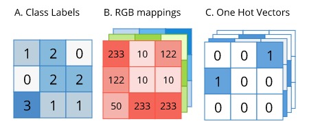
Labels for semantic segmentation are of the same size as of the original image. The label can be represented in one-hot encoded form as depicted below:

One-Hot format for semantic segmentation. ( Source )

Since the label is in a convenient one-hot form, it can be directly used as the ground truth (target) for calculating cross-entropy. However, softmax must be applied pixel-wise on the predicted output before applying cross entropy, as each pixel can belong to any one our target classes.

Focal Loss

Focal Loss, introduced in the RetinaNet paper proposes an upgrade to the standard cross-entropy loss for usage in cases with extreme class imbalance.

Consider the plot of the standard cross entropy loss equation as shown below (Blue color). Even in the case where our model is pretty confident about a pixel’s class (say 80%), it has a tangible loss value (here, around 0.3). On the other hand, Focal Loss (Purple color, with gamma=2 )does not penalize the model to such a large extent when the model is confident about a class (i.e. loss is nearly 0 for 80% confidence).

Standard Cross Entropy (Blue) vs Focal Loss with various values of gamma. ( Source )

Let us explore why this is significant with an intuitive example. Assume we have an image with 10000 pixels, with only two classes: Background class (0 in one-hot form) and Target class (1 in one-hot form). Let us assume 97% of the image is the background and 3% of the image is the target. Now, say our model is 80% sure about pixels that are background, but only 30% sure about pixels that are the target class.

While using cross-entropy, loss due to background pixels is equal to (97% of 10000) * 0.3 which equals 2850 and loss due to target pixels is equal to (3% of 10000) * 1.2 which equals 360 . Clearly, the loss due to the more confident class dominates, and there is very low incentive for the model to learn the target class. Comparatively, with focal loss, loss due to background pixels is equal to (97% of 10000) * 0 which is 0. This allows the model to learn the target class better.

Dice Loss

Dice Loss is another popular loss function used for semantic segmentation problems with extreme class imbalance. Introduced in the V-Net paper, the Dice Loss is used to calculate the overlap between the predicted class and the ground truth class. The Dice Coefficient (D) is represented as follows:

Dice Coefficient. ( Source )

Our objective is to maximize the overlap between the predicted and ground truth class (i.e. to maximize the Dice Coefficient). Hence, we generally minimize (1-D) instead to obtain the same objective, as most ML libraries provide options for minimization only.

Derivative of Dice Coefficient. ( Source )

Even though Dice Loss works well for samples with class imbalance, the formula for calculating its derivative (shown above) has squared terms in the denominator. When those values are small, we could get large gradients, leading to training instability.

Applications

Semantic Segmentation is used in various real life applications. Following are some of the significant use cases of semantic segmentation.

Autonomous Driving

Semantic segmentation is used to identify lanes, vehicles, people and other objects of interest. The resultant is used to make intelligent decisions to guide the vehicle properly.

Semantic segmentation for autonomous vehicles. ( Source )

One constraint on autonomous vehicles is that performance must be real time. A solution to the above problem is to integrate a GPU locally along with the vehicle. To enhance performance of the above solution, lighter (low parameters) neural networks can be used or techniques to fit neural networks on the edge can be implemented.

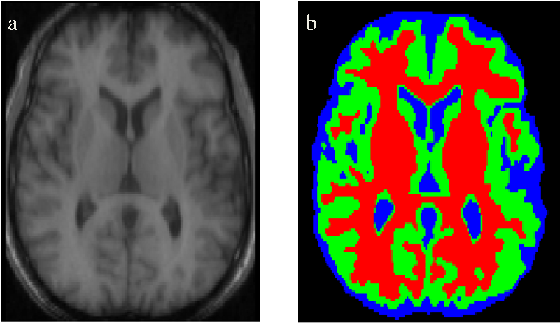
Medical Image Segmentation

Semantic Segmentation is used to identify salient elements in medical scans. It is especially useful to identify abnormalities such as tumors. The accuracy and low recall of algorithms are of high importance for these applications.

Segmentation of medical scans. ( Source )

We can also automate less critical operations such as estimating the volume of organs from 3D semantically segmented scans.

Scene Understanding

Semantic segmentation usually forms the base for more complex tasks such as Scene Understanding and Visual Question and Answer (VQA). A scene graph or a caption is usually the output of scene understanding algorithms

Scene Understanding in action. ( Source )

Fashion Industry

Semantic Segmentation is used in the Fashion Industry to extract clothing items from an image to provide similar suggestions from retail shops. More advanced algorithms can “re-dress” particular items of clothing in an image.

Semantic segmentation used as an intermediate step to redress a human based on text input. ( Source )

Satellite (Or Aerial) Image Processing

Semantic Segmentation is used to identify types of land from satellite imagery. Typical use cases involve segmenting water bodies to provide accurate map information. Other advanced uses cases involve mapping roads, identifying types of crops, identifying free parking space and so on.

Semantic segmentation of satellite/aerial images. ( Source )

Conclusion

Deep Learning greatly enhanced and simplified Semantic Segmentation algorithms and paved the way for greater adoption in real-life applications. The concepts listed in this blog are not exhaustive as research communities continuously strive to enhance the accuracy and real-time performance of these algorithms. Nevertheless, this blog introduces some popular variants of these algorithms and their real-life applications.