Every 7.8μs your computer’s memory has a hiccup

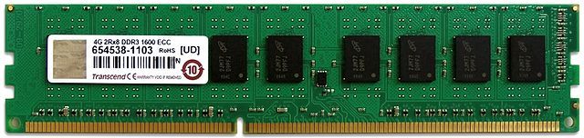Modern DDR3 SDRAM. Source: BY-SA/4.0 by Kjerish

During my recent visit to the Computer History Museum in Mountain View, I found myself staring at some ancient magnetic core memory .

Source: BY-SA/3.0 by Konstantin Lanzet

I promptly concluded I had absolutely no idea on how these things could ever work. I wondered if the rings rotate (they don't), and why each ring has three wires woven through it (and I still don’t understand exactly how these work). More importantly, I realized I have very little understanding on how the modern computer memory - dynamic RAM - works!

Source: Ulrich Drepper's series about memory

I was particularly interested in one of the consequences of how dynamic RAM works. You see, each bit of data is stored by the charge (or lack of it) on a tiny capacitor within the RAM chip. But these capacitors gradually lose their charge over time. To avoid losing the stored data, they must regularly get refreshed to restore the charge (if present) to its original level. This refresh process involves reading the value of every bit and then writing it back. During this "refresh" time, the memory is busy and it can't perform normal operations like loading or storing bits.

This has bothered me for quite some time and I wondered... is it possible to notice the refresh delay in software?

Dynamic RAM refresh primer

Each DIMM module is composed of "cells" and "rows", "columns", "sides" and/or "ranks". This presentation from the University of Utah explains the nomenclature . You can check the configuration of memory in your computer with decode-dimms command. Here's an example:

$ decode-dimms
Size                                       4096 MB
Banks x Rows x Columns x Bits              8 x 15 x 10 x 64
Ranks                                      2

For today we don't need to get into the whole DDR DIMM layout, we just need to understand a single memory cell, storing one bit of information. Specifically we are only interested in how the refresh process is performed.

Let's review two sources:

• A DRAM Refresh Tutorial, from the University of Utah
• And an awesome documentation of 1 gigabit cell from micron: TN-46-09 Designing for 1Gb DDR SDRAM

Each bit stored in dynamic memory must be refreshed, typically every 64ms (called Static Refresh). This is a rather costly operation. To avoid one major stall every 64ms, this process is divided into 8192 smaller refresh operations. In each operation, the computer’s memory controller sends refresh commands to the DRAM chips. After receiving the instruction a chip will refresh 1/8192 of its cells. Doing the math - 64ms / 8192 = 7812.5 ns or 7.81 μs. This means:

• A refresh command is issued every 7812.5 ns. This is called tREFI.
• It takes some time for the chip to perform the refresh and recover so it can perform normal read and write operations again. This time, called tRFC is either 75ns or 120ns (as per the mentioned Micron datasheet).

When the memory is hot (>85C) the memory retention time drops and the static refresh time halves to 32ms, and tREFI falls to 3906.25 ns.

A typical memory chip is busy with refreshes for a significant fraction of its running time - between 0.4% to 5%. Furthermore, memory chips are responsible for a nontrivial share of typical computer's power draw, and large chunk of that power is spent on performing the refreshes.

For the duration of the refresh action, the whole memory chip is blocked. This means each and every bit in memory is blocked for more than 75ns every 7812ns. Let's measure this.

Preparing an experiment

To measure operations with nanosecond granularity we must write a tight loop, perhaps in C. It looks like this:

for (i = 0; i < ...; i++) {
        __m128i x;
        // Perform data load. MOVNTDQA is here only for kicks,
        // for writeback memory it makes zero difference, the
        // caches are still polluted.
        asm volatile("movntdqa (%1), %0" :  "=x" (x) : "a" (one_global_var));


        // Lie to compiler to prevent optimizing this code. Claim that 'x' is referred to.
      asm volatile("" : : "x" ( x ));

              // Flush the value from CPU caches, to force memory fetch next time.
        _mm_clflush(one_global_var);

             // Measure and record time
       clock_gettime(CLOCK_MONOTONIC, &ts);
    }

Full code is available on Github .

The code is really straightforward. Perform a memory read. Flush data from CPU caches. Measure time.

I'm attempting to use MOVNTDQA to perform the data load, but this is not important. In fact, current hardware ignores the non-temporary load hint on writeback memory . In practice any memory load instruction would do.

On my computer it generates data like this:

# timestamp, loop duration
3101895733,     134
3101895865,     132
3101896002,     137
3101896134,     132
3101896268,     134
3101896403,     135
3101896762,     359
3101896901,     139
3101897038,     137

Typically I get ~140ns per loop, periodically the loop duration jumps to ~360ns. Sometimes I get odd readings longer than 3200ns.

Unfortunately, the data turns out to be very noisy. It's very hard to see if there is a noticeable delay related to the refresh cycles.

Fast Fourier Transform

At some point it clicked. Since we want to find a fixed-interval event, we can feed the data into the FFT (fast fourier transform) algorithm, which deciphers the underlying frequencies.

I'm not the first one to think about this - Mark Seaborn of Rowhammer fame implemented this very technique back in 2015. Even after peeking at Mark's code, getting FFT to work turned out to be harder than I anticipated. But finally I got all the pieces together.

First we need to prepare the data. FFT requires input data to be sampled with a constant sampling interval. We also want to crop the data to reduce noise. By trial and error I found the best results are when data is preprocessed:

• Small (smaller than average * 1.8) values of loop iterations are cut out, ignored, and replaced with readings of "0". We really don't want to feed the noise into the algorithm.
• All the remaining readings are replaced with "1", since we really don't care about the amplitude of the delay caused by some noise.
• I settled on sampling interval of 100ns, but any number up to a Nyquist value (double expected frequency) also work fine .
• The data needs to be sampled with fixed timings before feeding to FFT. All reasonable sampling methods work ok, I ended up doing basic linear interpolation.

The algorithm is roughly:

UNIT=100ns
A = [(timestamp, loop_duration),...] 
p = 1
for curr_ts in frange(fist_ts, last_ts, UNIT):
    while not(A[p-1].timestamp <= curr_ts < A[p].timestamp):
        p += 1
    v1 = 1 if avg*1.8 <= A[p-1].duration <= avg*4 else 0
    v2 = 1 if avg*1.8 <= A[p].duration <= avg*4 else 0
    v = estimate_linear(v1, v2, A[p-1].timestamp, curr_ts, A[p].timestamp)
    B.append( v )

Which on my data produces fairly boring vector like this:

[0, 0, 0, 0, 0, 0, 1, 0, 0, 0, 0, 0, 0, 0, 0, 0, 0, 0, 
 0, 0, 0, 0, 0, 0, 0, 0, 0, 0, 0, 0, 0, 0, 0, 1, 1, 0,
 0, 0, 0, 0, 0, 0, 0, 0, 0, 0, 0, 0, 0, 0, 0, 0, 0, 0, 
 0, 0, 1, 0, 0, 0, 0, 0, 0, 0, 0, 0, 0, 0, 0, 0, 0, 0, ...]

The vector is pretty long though, typically about ~200k data points. With data prepared like this, we are ready to feed it into FFT!

C = numpy.fft.fft(B)
C = numpy.abs(C)
F = numpy.fft.fftfreq(len(B)) * (1000000000/UNIT)

Pretty simple, right? This produces two vectors:

abs()

The result can be charted:

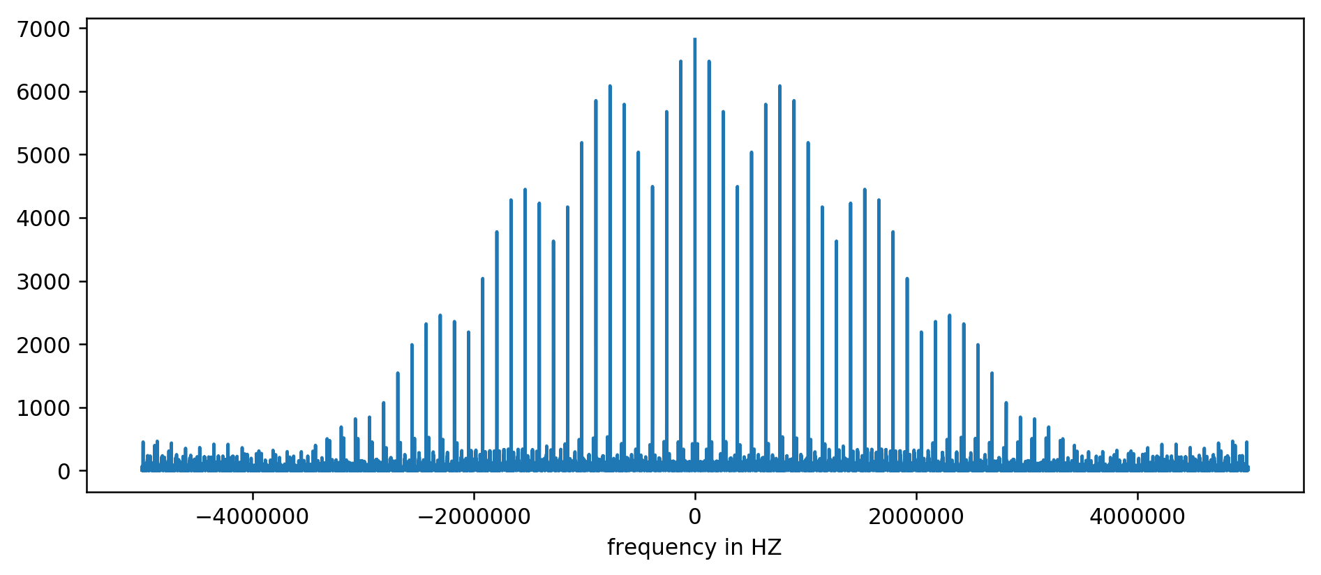
X axis is unit-less since we normalized the delay times. Even though, it clearly shows spikes at some fixed frequency intervals. Let's zoom in:

We can clearly see first three spikes. After a bit of wishy-washy arithmetic, involving filtering the reading at least 10 times the size of average, we can extract the underlying frequencies:

127850.0
127900.0
127950.0
255700.0
255750.0
255800.0
255850.0
255900.0
255950.0
383600.0
383650.0

Doing the math: 1000000000 (ns/s) / 127900 (Hz) = 7818.6 ns

Hurray! The first frequency spike is indeed what we were looking for, and indeed does correlate with the refresh times.

The other spikes at 256kHz, 384kHz, 512kHz and so on, are multiplies of our base frequency of 128kHz called harmonics. These are a side effect of performing FFT on something like a square wave and totally expected.

For easier experimentation, we prepared a command line version of this tool. You can run the code yourself. Here is a sample run on my server:

~/2018-11-memory-refresh$ make
gcc -msse4.1 -ggdb -O3 -Wall -Wextra measure-dram.c -o measure-dram
objdump -dx measure-dram | egrep 'movntdqa' -A 2 -B 2
 a29:    0f 1f 80 00 00 00 00     nopl   0x0(%rax)
 a30:    4c 89 e0                 mov    %r12,%rax
 a33:    66 0f 38 2a 00           movntdqa (%rax),%xmm0
 a38:    41 0f ae 3c 24           clflush (%r12)
 a3d:    0f ae f0                 mfence
./measure-dram | python3 ./analyze-dram.py
[*] Verifying ASLR: main=0x555555554890 stack=0x7fffffefe2ec
[ ] Fun fact. I did 40663553 clock_gettime()'s per second
[*] Measuring MOVNTDQA + CLFLUSH time. Running 131072 iterations.
[*] Writing out data
[*] Input data: min=117 avg=176 med=167 max=8172 items=131072
[*] Cutoff range 212-inf
[ ] 127849 items below cutoff, 0 items above cutoff, 3223 items non-zero
[*] Running FFT
[*] Top frequency above 2kHz below 250kHz has magnitude of 7716
[+] Top frequency spikes above 2kHZ are at:
127906Hz    7716
255813Hz    7947
383720Hz    7460
511626Hz    7141

I must admit the code is not perfectly stable. In case of trouble, consider disabling Turbo Boost, CPU frequency scaling and tuning for performance.

Finale

There are two major takeaways from this work.

We've seen that the low level data is pretty hard to analyze and seem to be pretty noisy. Instead of trying to figure something out with naked eye, we can always employ good old FFT. Some wishful thinking is needed when preparing the data.

Most importantly, we showed it's often possible to measure subtle hardware behaviours from a simple userspace process. This kind of thinking led to the discovery of the original Rowhammer vulnerability, was used in Meltdown/Spectre attacks and showed again in recent ECC-defeating reincarnation of Rowhammer .

There is so much more to be said. We barely scratched the surface of the inner workings of the memory subsystem. I recommend further reading:

• L3 cache mapping on Sandy Bridge CPUs
• How physical address maps to rows and banks in DRAM
• Hannu Hartikainen hacking DDR3 SO-DIMM to work... slower

Finally, here is a good reading about the old magnetic core memory:

• PDP-11 core memory explained by University of Sydney