Machine Learning: End-to-end Classification [FREE]

In machine learning, classification is the task of predicting the class of an object out of a finite number of classes, given some input labeled dataset. For example, you might have a list of 10,000 emails and the need to determine whether or not they’re spam. You would train a classifier on this input data and it would be able to predict if a new email is spam or not. Another classic example is a classifier that can predict what object is depicted in an image from a list of known classes such as house, car, cat and so on.

In this tutorial, you’ll learn how to:

• Preprocess and prepare data to feed into a machine learning classification algorithm.
• Evaluate your classifier against the most commonly used classification metrics.
• Optimize the parameters of a machine learning classifier.

Getting Started

Note : This tutorial requires having Jupyter Notebook and several Python scientific libraries used for machine learning training. If you don’t have these tools installed, please follow the first section of Beginning Machine Learning with scikit-learn . The relevant parts are Installing Anaconda , Installing Core ML Community Tools , and Jupyter Notebook .

Downloaded the materials for this tutorial using the Download Materials button at the top or bottom of this page. Copy the two ipynb files to your Jupyter Notebooks folder. Then, open Starter.ipynb with Jupyter.

From the top menu of Jupyter, select Kernel , and then Restart & Run All :

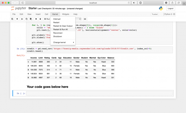
Select Restart and Run All Cells if prompted to “Restart kernel and re-run the whole notebook”.

The bottom cell contains code to download a dataset called credit. This dataset contains 400 rows wherein each row contains some credit-related information about a person as well as some personal details such as age and student status. You can see the first 5 rows in the notebook.

Your goal in this project is to use this dataset to create a classifier to predict whether or not a user is creditworthy, using as little personal information as possible. You define a creditworthy person as someone who has a credit score (rating) of over 600.

Preprocessing and Selecting Features

The first step to any machine learning project is cleaning or transforming the data into a format that can be used by machine learning algorithms. In most cases, you’ll need numerical data without any missing values or outliers that might make it much harder to train a model.

In the case of the credit dataset, the values are already very cleaned up, but you still need to transform the data into numerical values.

Encoding Labels

One of the simplest forms of preprocessing steps is called label encoding . It allows you to convert non numeric values to numeric values. You’ll use it to convert the Student, Married, and Gender columns.

Add the following code to a new cell just below, “Your code goes below here”:

# 1
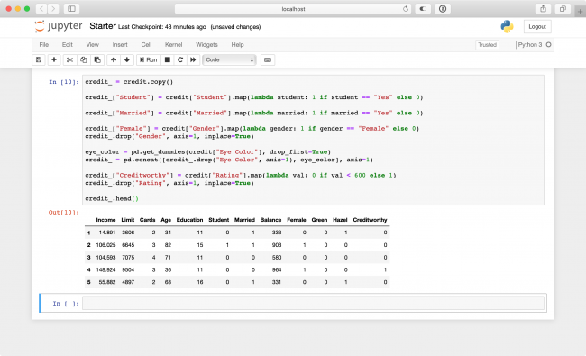
credit_ = credit.copy()

# 2
credit_["Student"] = credit["Student"].map(lambda student: 1 if student == "Yes" else 0)

credit_["Married"] = credit["Married"].map(lambda married: 1 if married == "Yes" else 0)

# 3
credit_["Female"] = credit["Gender"].map(lambda gender: 1 if gender == "Female" else 0)
credit_.drop("Gender", axis=1, inplace=True)

# 4
credit_.head()

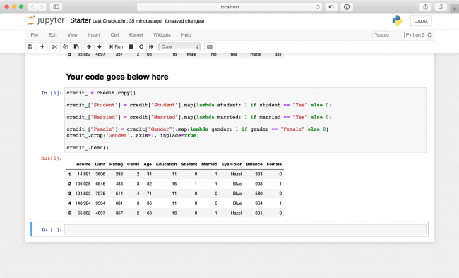
Here’s what’s happening in the code above:

1. You make a copy of the credit dataset to be able to cleanly transform the dataset. credit_ will hold the ready-to-use data after processing is complete.
2. For Student and Married , you label encode Yes to 1 and No to 0 .
3. Here, you also do the same for the Gender field, while renaming the column to Female . You also drop the Gender column afterwards.
4. At the end of the cell, you display the top rows from the data to verify your processing steps were successful.

Press Control+Enter to run your code. It should look similar to the following:

So far so good! You might be thinking about doing the same to the Eye Color column. This column holds three values: Green, Blue and Hazel. You could replace these values with 0, 1, and 2, respectively.

Most machine learning algorithms will misinterpret this information though. An algorithm like logistic regression would learn that Eye Color with value 2, will have a stronger effect than 1. A much better approach is using one-hot encoding.

One-Hot Encoding

When using one-hot encoding , also called Dummy Variables, you create as many columns as there are distinct values. Each column then becomes 0 or 1, depending on if the original value for that row was equal to the new column or not. For example, if the row’s value is Blue, then in the one-hot encoded data, the Blue column would be 1, then both the Green, and Hazel columns would be 0.

To better visualize this, create a new cell by choosing Insert ▸ Insert Cell Below from the top menu and add the following code to the new cell:

pd.get_dummies(credit_["Eye Color"])

get_dummies will create dummy variables from the values observed in Eye Color . Run the cell to check it out:

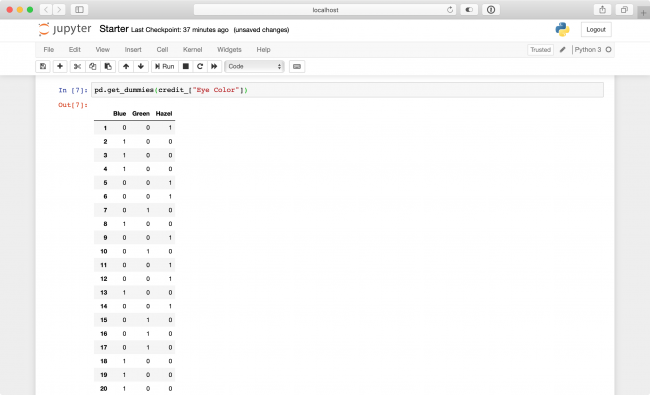
Because the first entry in your dataset had hazel eyes, the first result here contains a 1 in Hazel and 0 for Blue and Green. The remaining 399 entries work the same way!

Go to Edit ▸ Delete Cells to delete the last cell. Next, add the following lines just before credit_.head() in the latest cell:

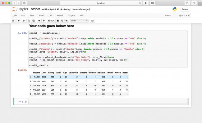
eye_color = pd.get_dummies(credit["Eye Color"], drop_first=True)
credit_ = pd.concat([credit_.drop("Eye Color", axis=1), eye_color], axis=1)

In the first line, you create the dummy columns for Eye Color while using drop_first=True to discard the first dummy column. You do this to save space because the last value can be inferred from the other two.

Then, you use concat to concatenate the dummy columns to the data frame at the end. Run the cell again and look at the results!

Target Label

For the last step of preprocessing, you’re going to create a target label. This will be the column your classifier will predict — in this case, whether or not the person is creditworthy.

For a Rating greater than 600, the label will be 1 (creditworthy). Otherwise, you set it to 0 . Add the following code to the current cell before credit_.head() again:

credit_["Creditworthy"] = credit["Rating"].map(lambda val: 0 if val < 600 else 1)
credit_.drop("Rating", axis=1, inplace=True)

This last column will be the column your classifier will predict, using a combination of the other columns.

Run this cell one last time. The preprocessing is now complete and your data frame is ready for training!

Training and Cross Validation

Now that the data is ready, you can create a classifier and train it. Add the following code to a new cell:

X = credit_[["Age", "Education", "Student", "Married"]]
y = credit_["Creditworthy"]

X_train, X_test, y_train, y_test = train_test_split(X, y, test_size=0.5, random_state=RANDOM_STATE)

You're selecting four of the features on which to train the model, and you are storing them in X . The Creditworthy column is your target, named y .

In the final line, you're splitting the dataset into two random halves, a training set to train the classifier on, and a testing set to validate the classifier to see how well you did. You can learn more about this process in the Beginning Machine Learning tutorial .

Next, add the following code to a new cell:

estimator = LogisticRegression(random_state=RANDOM_STATE)  # 1
estimator.fit(X_train, y_train)  # 2

y_true = y_test  # 3
y_pred = estimator.predict(X_test)  # 4
y_score = estimator.predict_proba(X_test)[:, 0]  # 5

There's a lot going on here:

1. You use logistic regression as the classifier. The details behind it are out of scope for this tutorial. You can learn more about this in this wonderful picture guide .
2. You train — or "fit" — the classifier on the training part of the dataset.
3. y_true will hold the true value of the y column that is the creditworthiness value. In this case, it's just the test values themselves.
4. y_pred holds the predicted new values of the creditworthiness. You'll use this value along with the true values to evaluate the performance of your classifier shortly. Note that this evaluation is done with the test set, because the classifier hasn't 'seen' these yet, and the goal is to predict unknown values. Otherwise, you could've just memorized the training values and predicted everything correctly every time.
5. Logistic regression is a classification algorithm that actually predicts a probability. The output of the model is something like: "The probability that the person with the given values is creditworthy is 75%." You can use these probability scores to evaluate more advanced metrics of the classifier.

You've successfully trained the classifier and used it to predict a probability! Next, you'll find out how well you did.

Accuracy

One of the simplest metrics to check how well you did is the accuracy of your model. What percentage of the values can the classifier predict correctly?

Add this line to a new cell:

accuracy_score(y_true=y_true, y_pred=y_pred)

accuracy_score takes your y column true and predicted values and returns the accuracy. Run the cell and check the results:

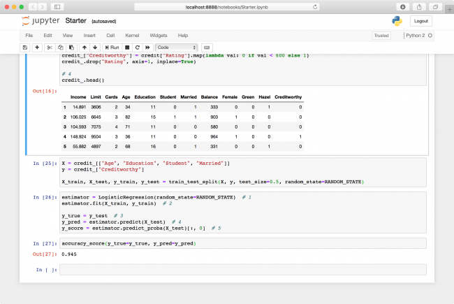
Almost 95%! Did you really do that well with just the age, education, student and marriage status of a person?

It turns out that out of the 200 rows in the testing dataset, only 11 of the rows are creditworthy. This means that a classifier that always predicts that the row is not creditworthy also has an accuracy of about 95%!

So the 95% your classifier predicted isn't that good — or any good actually. The accuracy, though often useful when the different classes are balanced, can be very misleading out of context. A better metric, or family of metrics, and one you should always look at, is the confusion matrix .

Understanding Confusion Matrix, Precision and Recall

A confusion matrix plots true values against predicted values. Precision and recall are two extremely useful metrics derived from a confusion matrix. In the context of your dataset, the metrics answer the following questions:

1. Precision : Out of all of the people who were creditworthy, what percentage of them were correctly predicted to be creditworthy?
2. Recall : Out of all of the people who were predicted to be creditworthy, what percentage of them were actually creditworthy?

This will become a bit clearer when you see the data, so it's time to add some code. Create new cells for each of the following code blocks and run them all (don't worry about the warning):

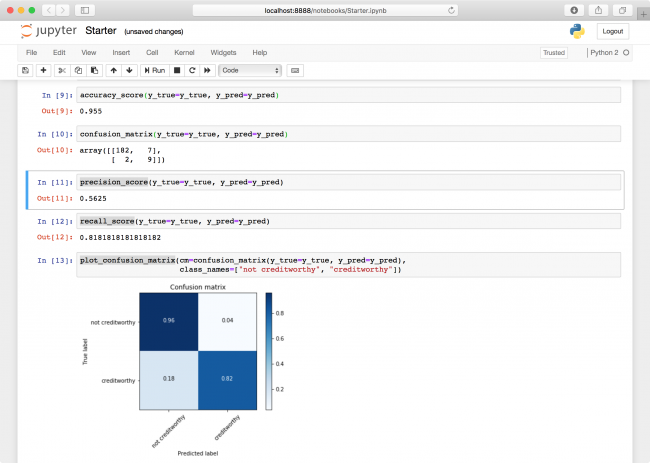
confusion_matrix(y_true=y_true, y_pred=y_pred)

precision_score(y_true=y_true, y_pred=y_pred)

recall_score(y_true=y_true, y_pred=y_pred)

plot_confusion_matrix(cm=confusion_matrix(y_true=y_true, y_pred=y_pred),
                      class_names=["not creditworthy", "creditworthy"])

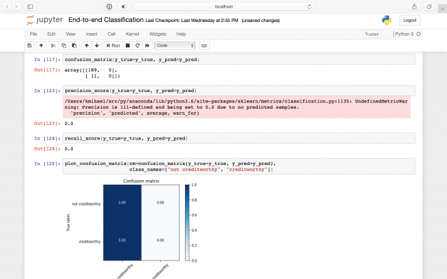
In the first cell, confusion_matrix plots the true values against the predicted values. Each quadrant in the output multi-dimensional array represents a combination of a true value and a predicted value . For example, the top-right is the number of rows that were not creditworthy and were also correctly predicted by your classifier to be not creditworthy.

The last cell includes a visualization of this, wherein each quadrant was also divided by the total number of rows. You can see that your current classifier is actually doing what you feared it was doing: It's just predicting all the rows to be not creditworthy.

In the middle, you'll see calculations for precision_score and recall_score . Both of these metrics range from 0 (0%) to 1 (100%). The closer you are to 1, the better. There's always a tradeoff between these two metrics.

For example, if you weren't as strict with your credit check, and you let some questionable people through, you would increase your precision, but your recall would suffer. On the other hand, if you were extremely strict, your recall might be impeccable, but you would fail to hand out credit to many creditworthy individuals, and your precision would suffer. The exact balance you need will depend on your use case.

Both your precision and your recall are 0, indicating that the classifier is currently quite terrible. Go back to the cell wherein you set X and y , and change X to the following:

X = credit_[["Income", "Education", "Student", "Married"]]

You're now using the Income value as part of the training. Go to Kernel ▸ Restart & Run All to re-run all of your cells.

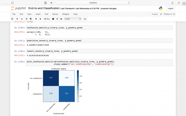
The precision has increased to 0.64 , and the recall to 0.81 ! This indicated that your classifier actually has some predictive power. Now you're getting somewhere.

Parameter tuning and pipelines

The logistic regression class has a couple of parameters you can set to further improve your classifier. Two useful ones are penalty , and C .

Which values should you set, though? Actually, why don't you try them all and see what works?

In the estimator cell, replace:

estimator = LogisticRegression(random_state=RANDOM_STATE)
estimator.fit(X_train, y_train)

With the following:

param_grid = dict(C=np.logspace(-5, 5, 11), penalty=['l1', 'l2'])
regr = LogisticRegression(random_state=RANDOM_STATE)
cv = GridSearchCV(estimator=regr, param_grid=param_grid, scoring='average_precision')
cv.fit(X_train, y_train)
estimator = cv.best_estimator_

Here, instead of using a default logistic regression with a C of 1.0 , and a penalty of l2 , you do an exhaustive search between 0.00001 to 100000 to see which yields a better precision in your classifier.

This grid search also accomplishes another very important task: It performs cross validation on your testing set. In doing so, it splits the testing set into smaller subsets and successively leaves a subset out of the training/evaluation. It then evaluates the precision of the classifier, and the final parameters it picks are the ones that yield the best average precision throughout all these subsets. This way, you can be much more confident that your classifier will be very robust and will yield similar results when used against unseen new data.

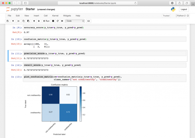
Run all the metrics cells again by going to Kernel ▸ Restart & Run All .

You'll see that the precision actually dropped down to 56%. The reason it dropped is that it's not really an apples-to-apples comparison, and you might have gotten lucky last time. The new precision you see is going to be closer to what you can expect "in the wild."

Scaling

Your classifier is already pretty good now, but you can still improve upon a precision of around 56%. One thing you always want to do is scale your dataset to be in the range of 0 to 1. Most classification algorithms will behave badly when datasets have columns with different scales of values. In this case, education ranges from 0 to 50, and income can be anywhere from 0 to virtually unlimited.

Replace the entire estimator cell with the following:

scaler = StandardScaler()  # 1
param_grid = dict(C=np.logspace(-5, 5, 11), penalty=['l1', 'l2'])
regr = LogisticRegression(random_state=RANDOM_STATE)
cv = GridSearchCV(estimator=regr, param_grid=param_grid, scoring='average_precision')
pipeline = make_pipeline(scaler, cv)  # 2

pipeline.fit(X_train, y_train)

# 3
y_true = y_test
y_pred = pipeline.predict(X_test)
y_score = pipeline.predict_proba(X_test)[:, 1]

Here's what this does:

1. You create a standard scaler.
2. You create a pipeline object that first scales the data and then feeds it into the grid search.
3. You can use the pipeline as if it were an estimator. You can call fit and predict on it, and it will even use the grid search's best estimator by default.

Run all the metrics cells again. The precision has increased to 72%!

ROC

Before wrapping up your classifier, there is one more metric you should always look at: ROC AUC . It is closely related to the confusion matrix, but also incorporates the predicted probabilities — or scores of a classifier. It ranges from 0 to 1 as well, where higher is better.

Intuitively, it measures how much better than random the score predictions are.

It does this by cutting off the probability scores at various thresholds and it rounds them down to make a prediction. It then plots the true positive rate — the rate of predicted creditworthy people who were actually creditworthy, or just the recall from above — against the false positive rate, which is the rate of predicted creditworthy people who were actually not creditworthy. This plot is called the ROC (receiver operating characteristic), and the metric ROC AUC (area under curve) is just the area under this curve!

Add the following code blocks to the bottom of your notebook into two new cells and run your cells one more time:

roc_auc_score(y_true=y_true, y_score=y_score)

plot_roc_curve(y_true=y_true, y_score=y_score)

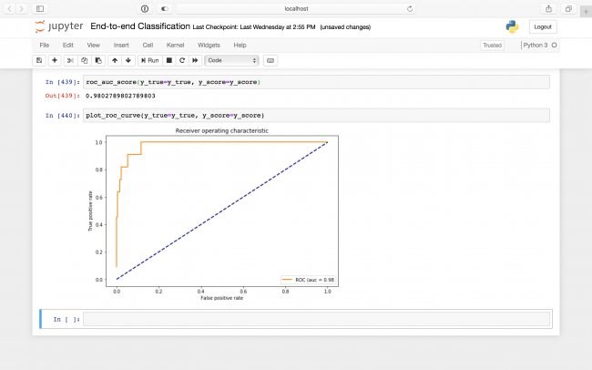
A ROC of 0.98 indicates your predictions are quite good!

Where to Go From Here?

Congratulations! You just trained an entire classifier; great job.

This tutorial has provided you with some of the most commonly used strategies you'll come across when working on your own classification problem.

The final notebook, included in the materials for this tutorial, also includes code to export a CoreML model from your classifier, ready to drop right into an iOS application.

Experiment with different combinations of input parameters, classification algorithms , and metrics to tweak your model to perfection.

We hope you enjoyed this tutorial and, if you have any questions or comments, please join the forum discussion below!