深度网络之FishNet: A Versatile Backbone for Image, Region, and Pixel Level Prediction

精选原创

開心的猫 2022-12-14 12:39:58 博主文章分类：深度学习 ©著作权

文章标签 深度学习神经网络 2d 卷积 fish 文章分类 虚拟化云计算 阅读数136

FishNet: A Versatile Backbone for Image, Region, and Pixel Level Prediction

FishNet: A Versatile Backbone for Image, Region, and Pixel Level Prediction

一些理解
背景介绍

相关工作
深度残差网络的恒等映射和孤立卷积

FishNet结构细节

特征细化（图3b/c）

UR-block
DR-Block

设计细节

用于处理梯度传播问题的FishNet设计
上/下采样函数的选择
body和tail之间的桥梁模块

实验

图像分类

实验结果
消融研究

检测与分割

总结
相关代码
相关链接

深度网络之FishNet: A Versatile Backbone for Image, Region, and Pixel Level Prediction_卷积

原文存档https://www.yuque.com/lart/papers/fish，若文中有表述不合理的地方请指出
更新于2019-07-15 20:35:39，补充一些新的理解，稍微调整了下结构

这篇文章的研究思路是这样的：

不同任务（分类与分割、检测）需要的特征的分辨率是不同的：

分类要总结高级语义信息
检测、分割则需要有着高分辨率的高级语义信息

希望将这些任务进行统一，同时利用针对像素级、区域级、图像级任务设计的网络的优势，实现针对不同任务共同的增益
高层的富含语义信息、分辨率较高的特征很有用，但是直接应用在分类中效果比较差

可能破坏了分类任务需要的平移旋转不变性
可能分类任务需要较低的分辨率的特征

于是针对Hourglass模型附加一个下采样高分辨高级特征的结构，整体构成了一个鱼的结构——FishNet
但是网络加大了，需要考虑的问题也会增多，例如优化问题，也就是梯度更新问题

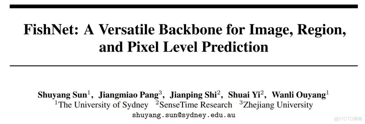
已有的有效的ResBlock结构，其附加的短连接有效的促进了梯度的回传与避免梯度消失的问题，但是在其结构中仍然存在一个不完美的地方，那就是用于调整尺寸和通道数的孤立卷积（Isolated Convolution），它的存在导致梯度不能无阻碍的直接回传
为什么过去的结构中这一缺点不明显呢？因为需要下采样的次数比较少，但是对于FishNet这样的结构，下采样更多，也就会需要考虑这个问题，更加极端的，在 Stacked Hourglass Networks中，会堆叠大量的hourglass结构，这个问题会更明显
FIshNet在网络设计中就尽可能去掉了这些孤立卷积，使用了一种更为“平滑”的方式降低梯度所受到的影响，使用池化来实现下采样，使用临近插值上采样，通道的调整可以使用拼接早期的特征以及分组缩减的设定来实现，这都是为了更好的进行梯度的回传

进一步考虑特征融合问题。对于特征之间的结合，现有的类似与FPN的结构，直接融合来自不同深度的信息。但是不同深度的特征有着对于图像内容的不同抽象程度，应该保留所有这些以改善特征的多样性。由于它们的互补性，它们可以用于相互细化

直接将来自高层和低层的特征相加（或者通过一些卷积处理后相加），得到的特征是混合后的特征，已经不再是原始的特征
高低层特征之间可以在保留（preserve）自身的情况下进行互相的细化（refine），而应避免混合（mix）
于是设计了FishNet中的DRBlock和URBlock（这一处知识点我开始没有注意到，后来再次听欧阳万里老师的讲解的时候才明白，原来有这样的考量），可以注意图中提到的信息提取的概念

网络整体结构也就出来了，可能会疑惑，如何使用这样的“整条鱼”来处理具体的分割任务呢，因为分类任务还直观些，可以直接使用最后的低分辨率的输出，那分割任务这样的需要高分辨率特征的，又该如何处理呢？（这里有必要问下作者，欧阳万里老师说是可以直接切掉鱼头，这样相较于原始的ResNet+FPN的效果要好，~~但是也说可以不切掉，这时如何处理，没有听明白，~~ 文中提到了在FishNet后添加FPN）

Object Detection Results Based on FPN. We report the results of detection using FPN with FishNet-150 on val-2017 for comparison.The top-down pathway and lateral connections（横向连接） in FPN are attached to the fish head.

整个网络最后可以端到端的训练，只在最后进行监督

设计用于预测不同级别（例如图像级，区域级和像素级）上的目标的卷积神经网络（CNN）结构的基本原理是不同的。

通常，专门用于图像分类的网络结构直接用作包括检测和分割在内的其他任务的默认骨干结构，但是考虑统一为像素级或区域级预测任务设计的情况下设计的骨干结构很少，这可能需要具有高分辨率的非常深的特征。为实现这一目标，设计了一个名为FishNet的网络。在FishNet中，所有分辨率的信息都会保留并针对最终任务进行细化。
此外，观察到现有的工作仍然不能直接将梯度信息从深层传播到浅层。该设计可以更好地解决这个问题。

已经进行了大量实验来证明FishNet的卓越性能。特别是在ImageNet-1k上，FishNet的精度能够以更少的参数超越DenseNet和ResNet的性能。FishNet被用作COCO Detection 2018挑战赛获奖作品中的一个模块。

深度网络之FishNet: A Versatile Backbone for Image, Region, and Pixel Level Prediction_卷积_02

本文结构主要由以下的三个优势：

这是第一个统一为像素级、区域级、图像级任务设计的骨干网络。 相较于纯粹为图像分类任务设计的网络，FishNet对于像素级和区域级任务而言更为有效。
它能够将梯度从非常深的层直接传播到较浅的层，这在文章中称为直接BP（direct BP）。 最近的工作表明，有两种设计可以实现直接BP，具有残余块和串联的恒等映射。然而，不言而喻的事实（unfold fact）是现有的网络设计，例如，ResNet和DenseNet等仍然不能够直接BP。此问题是由不同分辨率特征之间的卷积层引起的。

如图1所示，ResNet利用跳过连接上的带步幅的卷积层输入和输出通道数量或分辨率**的不一致，这使得_恒等映射不适用_。没有恒等映射或连接的卷积会降低从输出到浅层的梯度。
文章的设计通过将非常不同深度的特征连接到最终输出来更好地解决了这个问题。还仔细设计网络中的组件以确保直接BP。通过这些的设计，特征的语义信息也在整个网络中得以保留。

来自非常不同深度的特征被保留，并且用来互相细化。改善特征的多样性。由于它们的互补性，它们可以用于相互细化。

因此，文章设计了一种特征的保留和细化机制来实现这一目标。

# ResNet中的处理通道和分辨率不同的映射连接
if stride != 1 or self.inplanes != planes * block.expansion:
downsample = nn.Sequential(
conv1x1(self.inplanes, planes * block.expansion, stride),
nn.BatchNorm2d(planes * block.expansion),
)

文章设计的一个可能违反直觉的效果是它 在参数数量和图像分类精度之间的权衡中比传统的卷积网络表现更好。原因如下：

保留和细化的特征相互补充，比设计宽度或深度更大的网络更有用；
促进直接BP。实验结果表明，紧凑型FishNet-150，其参数数量接近ResNet-50：

能够超越ImageNet-1k上的ResNet-101和DenseNet-161（k = 48）的精度。
对于区域和像素级任务，如对象检测和实例分割，我们的模型作为Mask R-CNN的主干，与基线ResNet50相比，MS COCO上的绝对AP分别提高了2.8％和2.3％。

CNN architectures for image classification： 高分辨率的深层特征有着高级语义信息，并且同时可以提升图像分类任务的准确率。
Design in combining features from different layers： 之前的例如hyper-column、hourglass和fpn等的工作，虽然利用了来自深层和浅层的特征，但是并没有用来互相细化。常用于融合的操作有 add ，但这只是混合了不同抽象等级的特征，并不能保留或者互相细化，而 cat+conv 的操作和 add 的操作是类似的。当残差块（也带有加法）用于组合特征时，现有工作具有待细化的预定义目标。如果跳过层用于深层特征，则浅层特征仅用于细化深层特征，在残差块之后会被丢弃。总之，现有工程中的加法和残差块不会保留浅层和深层的特征，而文章的设计会保留和细化它们。
Networks with up-sampling mechanism： 由于计算机视觉中还有许多其他任务，例如对象检测，分割，需要大特征映射来保持分辨率：

有必要将上采样方法应用于网络。这种机制通常用于 具有非常不同深度的特征之间的通信。包括U-Net，FPN，堆叠hourglass等在内的一系列作品都在像素级任务和区域级任务中展示了它们的能力。但是，它们都没有被证明对图像分类任务有效。
MSDNet(Multi-Scale Dense Convolutional Networks，黄高)试图保持大分辨率的特征映射，这是文中架构最相似的工作。

但是，MSDNet的体系结构仍然使用不同分辨率的特征之间的卷积，这不能保留表示。
此外，它没有提供上采样途径来实现具有大分辨率和更多语义含义的特征。
MSDNet将多尺度机制引入其架构的目的是进行预算预测（do budget prediction）。然而，这种设计没有显示出图像分类精度的提高。

FishNet是第一个证明U-Net结构可以有效进行图像分类的网络。此外，为最终任务保留和优化浅层和深层的特征，这 在具有上采样或MSDNet的现有网络中是无法实现的。

Message passing among features/outputs： 有一些方法使用特征之间的消息传递进行分割，姿态估计和目标检测。这些设计基于骨干网络，FishNet是与它们互补的骨干网络。

深度残差网络的恒等映射和孤立卷积

ResNet的基础构建单元是残差块，有着恒等映射的残差块可以表示为：

深度网络之FishNet: A Versatile Backbone for Image, Region, and Pixel Level Prediction_2d_03

这里的xl表示输入特征，这里表示的是第l层的残差块。并且F表示残差函数，有着输入xl，和参数Wl。这里认为所有相同分辨率残差块的堆叠为一个阶段“stage”。阶段s中的第l层的特征表示为xl,s，所以有如下的关系：

深度网络之FishNet: A Versatile Backbone for Image, Region, and Pixel Level Prediction_神经网络_04

这里的Ls表示阶段s中堆叠的残差块的数量，L是损失函数。（2）中的附加项

深度网络之FishNet: A Versatile Backbone for Image, Region, and Pixel Level Prediction_神经网络_05

保证了xLs,s的梯度可以被直接传播到x0,s上。

在原始的ResNet中，考虑到不同分辨率的特征有着不同的通道数。因此一个过渡函数h()需要在下采样之前改变通道数：

深度网络之FishNet: A Versatile Backbone for Image, Region, and Pixel Level Prediction_2d_06

这里的sigma表示激活函数，lambda表示滤波器，bLs,s表示偏置，这都是阶段s中的参数，而其中的圈叉运算符表示卷积操作。因为输入的xLs,s和输出的x’0,s+1通道数不同，所以恒等映射不再适用。

所谓的 孤立（Isolated）卷积（I-conv） 是式子3中的卷积，没有恒等映射或连接。通过[Identity mappings in deep residual networks]中的实验分析和验证，希望将深层的梯度直接传输到浅层。具有恒等映射的残差块[Identity mappings in deep residual networks]和具有串联的密集块[Densely connected convolutional networks]促进了这种直接梯度传播。

如果存在I-conv，则深层的梯度不能直接传输到浅层。 然而，ResNet中不同分辨率的特征之间以及相邻密集块之间的I-conv（在[DenseNet]中称为过渡层）阻碍了直接梯度传播。

由于ResNet和DenseNet仍然具有I-conv，因此输出的梯度不能直接传播到它们的浅层，类似于[Imagenet classification with deep convolutional neural networks，Very deep convolutional networks for large-scale image recognition]中的网络。
[i-revnet: Deep invertible networks]中的可逆下采样通过使用当前阶段的所有特征用于下一阶段来避免I-conv的问题。问题是随着阶段ID的增加，它会以指数方式增加参数的数量（[i-revnet: Deep invertible networks]中为188M）。

已经在现有网络中确定了I-conv的梯度传播问题。因此，提出了一种新的架构，即FishNet，来解决这个问题。

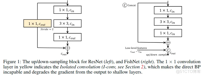
FishNet结构细节

深度网络之FishNet: A Versatile Backbone for Image, Region, and Pixel Level Prediction_2d_07

这里显示了FishNet的结构，整个网络分为了三个部分，tail，body，head。

tail是现有的CNN，例如ResNet，随着网络的深入，特征分辨率逐渐减小。
body则是有着数个上采样和细化块的结构，主要用来细化来自tail和body的特征。
head则是有着数个下采样和细化块的结构，用来保留和细化来自tail，body和head的特征。最后一个卷积层的细化特征被用来应对最终的任务。

本文中的”阶段“（stage）是指由具有相同分辨率的特征馈送的一堆卷积块。根据输出特征的分辨率，FishNet中的每个部分可以分为几个阶段。 随着分辨率变小，阶段ID变得更高。例如，输出分辨率为56x56和28x28的块分别位于FishNet的所有三个部分的第1和第2阶段。因此，在鱼尾和头部，阶段ID在前向传播时变得更高，而在身体部分中ID越来越小。

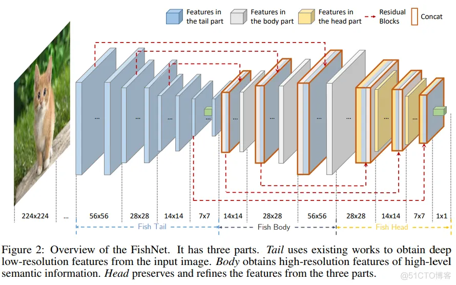
深度网络之FishNet: A Versatile Backbone for Image, Region, and Pixel Level Prediction_2d_08

图3显示了两个阶段特征的尾部，身体和头部之间的相互作用。

图3a中的tail可被视为残差网络。tail的特征经历（undergo）几个残余块并且还通过水平箭头传递到nody。
图3a中的body通过连接保留了尾部的特征和身体前一阶段的特征。然后，这些连接的特征将被上采样并细化，细节如b中所示。
对于head会使用前面细化的特征和之前的head的特征。head中的信息传递方式可见c。
在tail，body，head的水平连接表示之间的传递块。在图3a中， 使用残差块作为传输块。

特征细化（图3b/c）

FishNet中有两个特征细化模块，一个是3b中所示的UR-block和3c中所示的DR-block。

UR-block

该模块主要存在于body部分，所以其输入也就是来自于tail和body的特征。其表达式可以写成：

深度网络之FishNet: A Versatile Backbone for Image, Region, and Pixel Level Prediction_卷积_09

其中的xst和xsb表示来自tail和body的位于阶段s的第一层的特征。
由于这里是相同的分辨率之间互相关联，所以这里的s最小为1，最大为tail和body中阶段数N减去1后的小值。
式子里的τ表示的从tail到body之间传送特征xs-1t用的残差块。
这里的xs-1b表示从body上个阶段细化后得到的特征。

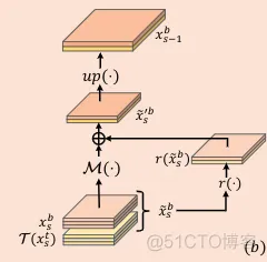
深度网络之FishNet: A Versatile Backbone for Image, Region, and Pixel Level Prediction_深度学习_10

具体细节： 从xst和xsb细化得到输出的过程表示如下：

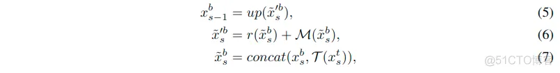
深度网络之FishNet: A Versatile Backbone for Image, Region, and Pixel Level Prediction_2d_11

特征使用了串联的方式进行了组合。
这里的up表示的上采样函数。顺序一次是7->6->5。得到这一阶段的输出。
式子中的M表示从特征提取信息的函数。这里使用卷积实现。相似于式子1中的残差函数F，这里的M使用ResNet中的Bottleneck单元实现，有着3个卷积层。
式子中的r表示通道级缩减函数可以表示为如下的关系，这是元素级加和，将k个通道关联到了一个通道上，这里将 通道缩减为原来的1/k，这使得可以降低计算和存储规模。

深度网络之FishNet: A Versatile Backbone for Image, Region, and Pixel Level Prediction_深度学习_12

深度网络之FishNet: A Versatile Backbone for Image, Region, and Pixel Level Prediction_卷积_13

表示有着cin通道的输入特征图，hatx表示有着cout通道的输出特征图，且有这关系cin/cout=k，所以等式中x(k*n+j)表示按照输入与输出的比例关系对输入的特征进行了一个分组，每个输出的通道只和其中的一组k个输入有关，是其中一组的加和。

DR-Block

而该模块主要用在head部分，相似于UR-block。只有两处不同：

使用2x2最大池化来下采样。
不使用通道缩减函数，以至于当前阶段的梯度可以直接被传送到先前的阶段。

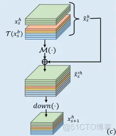
深度网络之FishNet: A Versatile Backbone for Image, Region, and Pixel Level Prediction_fish_14

具体细节： 从xsh和xsb得到xs+1h的过程表示如下：

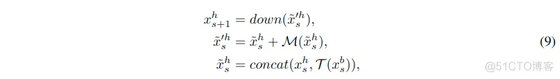
深度网络之FishNet: A Versatile Backbone for Image, Region, and Pixel Level Prediction_深度学习_15

符号表示类似。以这种方式，整个网络的每个阶段的特征都可以 通过串联、跳跃链接和最大池化的方式直接连接到最后一层。注意这里没有使用通道缩减操作r。因此从DR-block中获得hatxs’h的层可以被看作是残差块。

用于处理梯度传播问题的FishNet设计

在FishNet中设计了body和head，来自tail和body各个阶段的特征都在head串联起来。

仔细设计了head的层，这样就没有I-conv。head中的层由串联，带有恒等映射的卷积和最大池化组成。因此，FishNet解决尾部中先前那些骨干网络的梯度传播问题，主要通过：

排除head的I-conv
在body和head使用连接

上/下采样函数的选择

对于使用步幅2进行下采样，核为2x2以避免像素之间的重叠。消融研究将显示网络中不同类型内核大小的影响。

为了避免I-conv的问题，应该避免上采样方法中的加权反卷积。为简单起见，选择最近邻插值进行上采样。

个人理解：加权反卷积实际上就是在指代“反卷积”或者“转置卷积”的操作，这本身就是一种卷积操作，是一种I-Conv。并不利于梯度的传播。

由于 上采样操作会以较低的分辨率稀释（dilute）输入特征，因此在细化块中应用扩张卷积。

body和tail之间的桥梁模块

由于tail将对特征进行向下采样分辨率为1x1，因此需要将这1x1的特征上采样为7x7。在此处应用SE块以使用通道注意力操作，将特征从1x1映射到7x7。

For image classification, we evaluate our network on the ImageNet 2012 classification dataset that consists of 1000 classes.

1.2 million images for training
50000 images for validation (denoted by ImageNet-1k val)
All the experiments in this paper are evaluated through single-crop validation process its shorter side being resized to 256 This 224x224 image region is the input of the network.

Training:

randomly crop the images into the resolution of 224x224 with batch size 256
We follow the way of augmentation ( random crop, horizontal flip and standard color augmentation) used in [ResNet] for fair comparison.
stochastic gradient descent (SGD)
the base learning rate set to 0.1
weight decay and momentum are 1e-4 and 0.9 respectively
100 epochs
the learning rate is decreased by 10 times every 30 epochs
the normalization process is done by first converting the value of each pixel into the interval [0, 1], and then subtracting the mean and dividing the variance for each channel of the RGB respectively

由于FishNet是一个框架，并不制定构件块，对于本文的实验结果，FishNet使用的是带有恒等映射的残差块作为基础构建块，而FishNeXt则是使用带有恒等连接和分组的残差块作为构件块。

深度网络之FishNet: A Versatile Backbone for Image, Region, and Pixel Level Prediction_神经网络_16

When our network uses pre-activation ResNet as the tail part of the FishNet, the FishNet performs better than ResNet and DenseNet. （不是原始的ResNet，Conv-BN-ReLU的顺序有变化，所谓预激活）

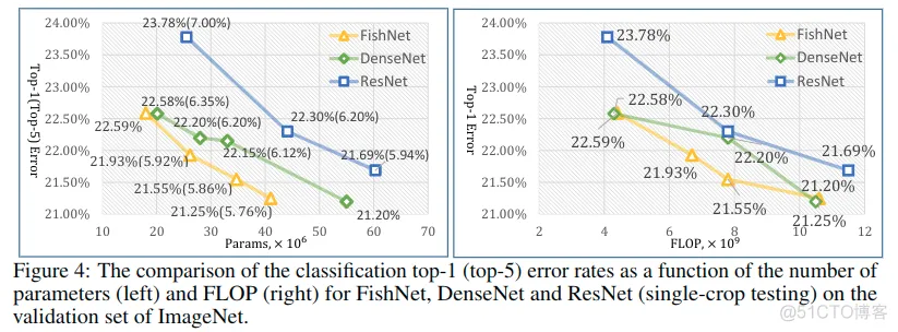
FishNet与ResNet： 为了公平比较，重现了ResNet，在图中汇报了结果，实际要比ResNet的论文结果要高，因为使用的是预激活残差块来作为基础构件块。可见，相比之下，FishNet实现了更高的指标，而且参数也相对更少，FishNet-150（21.93%，26.4M）的参数接近于ResNet-50（23.78%，25.5M），但是top1误差率低了。并且性能也超过了ResNet101（22.30%，44.5M）。在FLOPs上也实现了较好的表现。

FishNet与DenseNet： DenseNet通过串联迭代地聚合具有相同分辨率的特征，然后通过过渡层在每个dense块之间减小维度。根据图4中的结果，DenseNet能够使用更少的参数超过ResNet的精度。由于FishNet保留了更多样化的特征并且更好地处理了梯度传播问题，因此FishNet能够以更少的参数实现比DenseNet更好的性能。 此外，FishNet的内存成本也低于DenseNet。以FishNet-150为例，当单个GPU上的批量大小为32时，FishNet-150的内存成本为6505M，比DenseNet-161（9269M）小2764M。

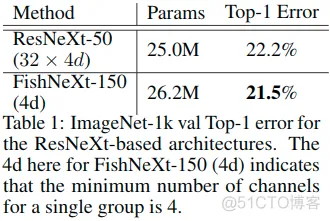
深度网络之FishNet: A Versatile Backbone for Image, Region, and Pixel Level Prediction_深度学习_17

FishNeXt与ResNeXt： FishNet的架构可以与其他类型的设计相结合，例如ResNeXt采用的通道分组。遵循以下标准： 同一级的每个块（UR / DR块和传输块）的组中的通道数应该相同。 一旦阶段索引增加1，单个组的宽度将加倍。这样，基于ResNet的FishNet可以构建为基于ResNeXt的网络，即FishNeXt。我们构建了一个具有2600万个参数的紧凑型FishNeXt-150。FishNeXt-150的参数数量接近ResNeXt-50。从表1可以看出，与相应的ResNeXt架构相比，绝对top1错误率可降低0.7％。

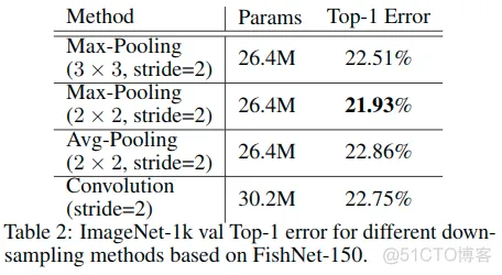
深度网络之FishNet: A Versatile Backbone for Image, Region, and Pixel Level Prediction_深度学习_18

池化与步幅卷积： 研究了基于FishNet-150的四种下采样方法，包括卷积、核为2x2和3x3的最大池化，以及核为2x2的平均池化。

如表2所示，应用2x2 max-pooling的性能优于其他方法。
Stride-Convolution将阻止（hinder）直接将损失梯度传播到浅层，而池化则不会。
还发现核为3x3的max-pooling比2x2更糟糕，因为结构信息可能受到具有重叠的池化窗口的3x3的最大池化的干扰。

When convolution with a stride of 2 is used, it is used for both the tail and the head of the FishNet.
When pooling is used, we still put a 1x1 convolution on the skip connection of the last residual blocks for each stage at the tail to change the number of channels between two stages, but we do not use such convolution at the head.

扩张卷积：[Dilated residual networks]发现 空间敏锐度的丧失可能导致图像分类准确性的限制。在FishNet中，UR-block将稀释原始的低分辨率特征，因此，在body部分中采用扩张卷积。

当在body上使用扩张卷积来上采样时，基于FishNet-150，绝对top1错误率降低0.13％。
然而，如果没有引入任何扩张的模型中，在body和head中使用扩张卷积，则绝对top1错误率增加0.1％。
此外，用两个残差块替换第一个7x7步幅卷积层，这将减少绝对top1个误差0.18％。

检测与分割

We evaluate the generalization capability of FishNet on object detection and instance segmentation on MS COCO. For fair comparison, all models implemented by ourselves use the same settings except for the network backbone. All the codes implementing the results reported in this paper about object detection and instance segmentation are released at [ https://github.com/open-mmlab/mmdetection].

数据集与指标：

There are 80 classes with bounding box annotations and pixel-wise instance mask annotations. It consists of：

118k images for training (train-2017)
5k images for validation (val-2017)
We train our models on the train-2017 and report results on the val-2017.

We evaluate all models with the standard COCO evaluation metrics AP (averaged mean Average Precision over different IoU thresholds), and the APS, APM, APL (AP at different scales).

深度网络之FishNet: A Versatile Backbone for Image, Region, and Pixel Level Prediction_fish_19

We re-implement the Feature Pyramid Networks (FPN) and Mask R-CNN based on PyTorch, and report the re-implemented results in Table 3.

Our re-implemented results are close to the results reported in Detectron[ https://github.com/facebookresearch/detectron].
With FishNet, we trained all networks on 16 GPUs with batch size 16 (one per GPU) for 32 epochs.
SGD is used as the training optimizer with a learning rate 0.02, which is decreased by 10 at the 20 epoch and 28 epoch.
As the mini-batch size is small, the batch-normalization layers in our network are all fixed during the whole training process.
A warming-up training process is applied for 1 epoch
The gradients are clipped below a maximum hyper-parameter of 5.0 in the first 2 epochs to handle the huge gradients during the initial training stage.
The weights of the convolution on the resolution of 224x224 are all fixed. We use a weight decay of 0.0001 and a momentum of 0.9.
The networks are trained and tested in an end-to-end manner. All other hyper-parameters used in experiments follow those in [ https://github.com/facebookresearch/detectron].

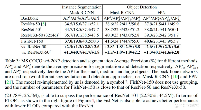
Object Detection Results Based on FPN. We report the results of detection using FPN with FishNet-150 on val-2017 for comparison. The top-down pathway and lateral connections（横向连接） in FPN are attached to the fish head. As shown in Table 3, the FishNet-150 obtains a 2.6% absolute AP increase to ResNet-50, and a 1.3% absolute AP increase to ResNeXt-50.

Instance Segmentation and Object Detection Results Based on Mask R-CNN. Similar to the method adopted in FPN, we also plug FishNet into Mask R-CNN for simultaneous segmentation and detection（同时分割和检测）. As shown in Table 3, for the task of instance segmentation, 2.3% and 1.3% absolute AP gains are achieved compared to the ResNet-50 and ResNeXt-50. Moreover, when the network is trained in such multi-task fashion, the performance of object detection could be even better. With the FishNet plugged into the Mask R-CNN, 2.8% and 1.5% improvement in absolute AP have been observed compared to the ResNet-50 and ResNeXt-50 respectively.

Note that FishNet-150 does NOT use channel-wise grouping, and the number of parameters for FishNet-150 is close to that of ResNet-50 and ResNeXt-50. When compared with ResNeXt-50, FishNet-150 only reduces absolute error rate by 0.2% for image classification, while it improves the absolute AP by 1.3% and 1.5% respectively for object detection and instance segmentation. This shows that the FishNet provides features that are more effective for the region-level task of object detection and the pixel-level task of segmentation.

COCO Detection Challenge 2018. FishNet was used as one of the network backbones of the winning entry. By embedding the FishNet into our framework, the single model FishNeXt-229 could finally achieve 43.3% on the task of instance segmentation on the test-dev set.

在本文中提出了一种新颖的CNN架构，以统一为在不同层次上识别目标的任务而设计的架构。 特征保留和细化的设计不仅有助于处理直接梯度传播的问题，而且对像素级和区域级任务也很友好。

实验结果证明并验证了网络的改进。对于未来的工作，将研究更详细的网络设置，例如每个阶段的通道/块数，以及与其他网络架构的集成。还将报告两个数据集上较大模型的性能。

# https://github.com/kevin-ssy/FishNet/blob/master/models/fishnet.py
'''
FishNet
Author: Shuyang Sun
'''
from __future__ import division

import math

import torch
import torch.nn as nn
from torchsummary import summary

class Bottleneck(nn.Module):
def __init__(self, inplanes, planes, stride=1, mode='NORM', k=1, dilation=1):
"""
基础残差块，用来构建整个网络的基石

:param inplanes: 输入通道数
:param planes: 输出通道数，若是不等于输入通道数，则使用孤立卷积进行处理
:param stride: 步长，决定这是否调整分辨率，若调整分辨率，则使用孤立卷积进行处理，
实际上代码中并没有使用非1的步长，所以这项没有太大的意义，使用的是双线性插值上采样和
最大迟化下采样进行的调整
:param mode: 快捷连接的模式
:param k: 上采样时，通道缩减比例
:param dilation: 扩张率
"""
super(Bottleneck, self).__init__()
self.mode = mode
# ReLU可以反复用，没必要多次定义
self.relu = nn.ReLU(inplace=True)
self.k = k

btnk_ch = planes // 4
# 1x1
self.bn1 = nn.BatchNorm2d(inplanes)
self.conv1 = nn.Conv2d(inplanes, btnk_ch, kernel_size=1, bias=False)
# 3x3 dilated
self.bn2 = nn.BatchNorm2d(btnk_ch)
self.conv2 = nn.Conv2d(btnk_ch, btnk_ch, kernel_size=3, stride=stride, padding=dilation,
dilation=dilation, bias=False)
# 1x1
self.bn3 = nn.BatchNorm2d(btnk_ch)
self.conv3 = nn.Conv2d(btnk_ch, planes, kernel_size=1, bias=False)

if mode == 'UP':
self.shortcut = None
elif inplanes != planes or stride > 1:
# 只有下采样的时候或者通道改变的时候使用孤立卷积
self.shortcut = nn.Sequential(
nn.BatchNorm2d(inplanes),
self.relu,
nn.Conv2d(inplanes, planes, kernel_size=1, stride=stride, bias=False)
)
else:
self.shortcut = None

def _pre_act_forward(self, x):
residual = x

out = self.bn1(x)
out = self.relu(out)
out = self.conv1(out)

out = self.bn2(out)
out = self.relu(out)
out = self.conv2(out)

out = self.bn3(out)
out = self.relu(out)
out = self.conv3(out)

if self.mode == 'UP':
# 只有上采样的时候，要降低通道，这里使用了分组融合的方式
residual = self.squeeze_idt(x)
elif self.shortcut is not None:
residual = self.shortcut(residual)

out += residual

return out

def squeeze_idt(self, idt):
n, c, h, w = idt.size()
# 注意这里分组融合的实现方式，实现了由c到c//self.k的过渡
return idt.view(n, c // self.k, self.k, h, w).sum(2)

def forward(self, x):
out = self._pre_act_forward(x)
return out

class Fish(nn.Module):
def __init__(self, block, num_cls=1000, num_down_sample=5, num_up_sample=3,
trans_map=(2, 1, 0, 6, 5, 4),
network_planes=None, num_res_blks=None, num_trans_blks=None):
"""
鱼形结构构造
:param block: 基础结构，这里使用的是一个预激活残差块
:param num_cls: 最终分类数量
:param num_down_sample: 下采样次数
:param num_up_sample: 上采样次数
:param trans_map: 还不清楚
:param network_planes: 网络各层通道数
:param num_res_blks: 各个位置残差块的数量
:param num_trans_blks: 各个位置传输块数量
"""
super(Fish, self).__init__()
self.block = block
self.trans_map = trans_map
self.upsample = nn.Upsample(scale_factor=2)
# 研究了四种下采样方法，包括卷积、核为2x2和3x3的最大池化，以及核为2x2的平均池化，其中2x2的最大池化效果最好
# When pooling is used, we still put a 1x1 convolution on the skip
# connection of the last residual blocks（涉及到了调整分辨率） for each
# stage at the tail to change the number of channels
# between two stages, but we do not use such convolution at the head.
self.down_sample = nn.MaxPool2d(2, stride=2)
self.num_cls = num_cls
self.num_down = num_down_sample
self.num_up = num_up_sample
self.network_planes = network_planes[1:]
self.depth = len(self.network_planes)
self.num_trans_blks = num_trans_blks
self.num_res_blks = num_res_blks
# 构建网络
self.fish = self._make_fish(network_planes[0])

def _make_score(self, in_ch, out_ch=1000, has_pool=False):
"""
BatchNorm2d-396 [-1, 2112, 7, 7] 4,224
ReLU-397 [-1, 2112, 7, 7] 0
Conv2d-398 [-1, 1056, 7, 7] 2,230,272
BatchNorm2d-399 [-1, 1056, 7, 7] 2,112
ReLU-400 [-1, 1056, 7, 7] 0
AdaptiveAvgPool2d-401 [-1, 1056, 1, 1] 0
Conv2d-402 [-1, 1000, 1, 1] 1,057,000
:param in_ch: 输入通道数
:param out_ch: 输出通道数
:param has_pool: 是否使用全局平均池化
:return: [conv, fc] 前者输出为in_ch//2，后者输出为out_ch
"""
bn = nn.BatchNorm2d(in_ch)
relu = nn.ReLU(inplace=True)
conv_trans = nn.Conv2d(in_ch, in_ch // 2, kernel_size=1, bias=False)
bn_out = nn.BatchNorm2d(in_ch // 2)
conv = nn.Sequential(bn, relu, conv_trans, bn_out, relu)

if has_pool:
fc = nn.Sequential(
nn.AdaptiveAvgPool2d(1),
nn.Conv2d(in_ch // 2, out_ch, kernel_size=1, bias=True)
)
else:
fc = nn.Conv2d(in_ch // 2, out_ch, kernel_size=1, bias=True)

# 因为上面的输出还要结合前面的传输过来的特征，所以这里还得将conv也输出
return [conv, fc]

def _make_se_block(self, in_ch, out_ch):
"""
构造了一个se通道注意力模块：
bn->relu->global_pool->conv1x1->relu->conv1x1->sigmoid
"""
bn = nn.BatchNorm2d(in_ch)
sq_conv = nn.Conv2d(in_ch, out_ch // 16, kernel_size=1)
ex_conv = nn.Conv2d(out_ch // 16, out_ch, kernel_size=1)
return nn.Sequential(bn,
nn.ReLU(inplace=True),
nn.AdaptiveAvgPool2d(1),
sq_conv,
nn.ReLU(inplace=True),
ex_conv,
nn.Sigmoid())

def _make_residual_block(self, inplanes, outplanes, nstage, is_up=False, k=1, dilation=1):
"""
在上下采样之后（如果需要的话），紧跟一系列残差块，后面这些通道是一致的。
:param inplanes: 输入的通道数
:param outplanes: 输出的通道数
:param nstage: 该部分要堆叠多少个残差块
:param is_up: 是否上采样
:param k: 上采样的时候通道压缩的比例
:param dilation: 除了上下采样部分后续残差块扩张率
:return: nn.Sequential(*layers) 一个堆叠的残差块序列
"""
layers = []

if is_up:
# 上采样的时候，要通道缩减，使用函数r
layers.append(self.block(inplanes, outplanes, mode='UP', dilation=dilation, k=k))
else:
# 其他的情况调整通道使用一个额外的孤立卷积
layers.append(self.block(inplanes, outplanes, stride=1))

# 每个阶段中的残差块除了调整维度的那一个残差块之外的其余残差块，这些都是直接的shortcut，同时，这些都是用扩张卷积的形式的
for i in range(1, nstage):
layers.append(self.block(outplanes, outplanes, stride=1, dilation=dilation))

return nn.Sequential(*layers)

def _make_stage(self, is_down_sample, inplanes, outplanes, n_blk, has_trans=True,
has_score=False, trans_planes=0, no_sampling=False, num_trans=2, **kwargs):
"""
构造阶段模块，阶段中的上下采样只是在最后输出的时候，考虑最大池化下采样还是双线性插值上采样
:param is_down_sample: 是否遭过程中进行下采样
:param inplanes: 输入的通道数，这里应该是已经拼接之后的输入通道数
:param outplanes: 输出的通道数
:param n_blk: 每个晓得残差块序列内部残差块的数量
:param has_trans: 是否有传输层
:param has_score: 是否有得分层
:param trans_planes: 传输通道
:param no_sampling: 是否有采样操作
:param num_trans: 传输数量
:param kwargs: 其他参数
:return: 阶段中的模块列表
"""
sample_block = []

if has_score:
sample_block.extend(self._make_score(outplanes, outplanes * 2, has_pool=False))

# 这里进行了上、下采样之前需要的通道的调整，在调整完后会进行一系列(算上上下采样部分总共有n_blk个)的残差块处理，只是通道数都是一致的
if no_sampling or is_down_sample:
# 对于阶段中的下采样，先进行残差块的构建，这里构建残差块，也就是M(+r)的步骤
res_block = self._make_residual_block(inplanes, outplanes, n_blk, **kwargs)
else:
# 上采样需要制定is_up，因为它有特殊的处理，需要进行通道缩减
res_block = self._make_residual_block(inplanes, outplanes, n_blk, is_up=True, **kwargs)
sample_block.append(res_block)

# 上下采样之前会考虑拼接的来自传输层和上一阶段的输出
# 上下采样之前的调整结束之后，会考虑来自传输层的特征，这里的num_trans表示传输层的残差块数量
if has_trans:
trans_in_planes = self.in_planes if trans_planes == 0 else trans_planes
sample_block.append(
self._make_residual_block(trans_in_planes, trans_in_planes, num_trans))

# 上下采样的部分，下采样使用的是最大迟化，上采样使用的是最邻近插值
if not no_sampling and is_down_sample:
sample_block.append(self.down_sample)
elif not no_sampling: # Up-Sample
sample_block.append(self.upsample)

return nn.ModuleList(sample_block)

def _make_fish(self, in_planes):
"""
构建不同阶段的模块
"""
def get_trans_planes(index):
"""获取传输层的通道数"""
map_id = self.trans_map[index - self.num_down - 1] - 1
p = in_planes if map_id == -1 else cated_planes[map_id]
return p

def get_trans_blk(index):
"""获取传输层的残差块数"""
return self.num_trans_blks[index - self.num_down - 1]

def get_cur_planes(index):
"""获取当前阶段的通道数"""
return self.network_planes[index]

def get_blk_num(index):
"""获取当前阶段的残差块数"""
return self.num_res_blks[index]

cated_planes, fish = [in_planes] * self.depth, []
for i in range(self.depth):
# even num for down-sample, odd for up-sample，根据奇偶索引确定上下采样
is_down = i not in range(self.num_down,
self.num_down + self.num_up + 1)
has_trans, no_sampling = i > self.num_down, i == self.num_down

cur_planes, trans_planes = get_cur_planes(i), get_trans_planes(i)
cur_blocks, num_trans = get_blk_num(i), get_trans_blk(i)

stg_args = [is_down, cated_planes[i - 1], cur_planes, cur_blocks]

if is_down or no_sampling:
k, dilation = 1, 1
else:
k, dilation = cated_planes[i - 1] // cur_planes, \
2 ** (i - self.num_down - 1)

# 构建阶段块
sample_block = self._make_stage(*stg_args,
has_trans=has_trans,
trans_planes=trans_planes,
has_score=(i == self.num_down),
num_trans=num_trans,
k=k,
dilation=dilation,
no_sampling=no_sampling)

if i == self.depth - 1:
# 在最后构建得分层
sample_block.extend(self._make_score(
cur_planes + trans_planes, out_ch=self.num_cls, has_pool=True
))
elif i == self.num_down:
# 构建收缩扩张阶段之间的se-block
sample_block.append(nn.Sequential(
self._make_se_block(cur_planes * 2, cur_planes)
))

if i == self.num_down - 1:
cated_planes[i] = cur_planes * 2
elif has_trans:
cated_planes[i] = cur_planes + trans_planes
else:
cated_planes[i] = cur_planes
fish.append(sample_block)
return nn.ModuleList(fish)

def _fish_forward(self, all_feat):
def _concat(a, b):
return torch.cat([a, b], dim=1)

def stage_factory(*blks):
"""
:param blks:
:return:
"""
def stage_forward(*inputs):
if stg_id < self.num_down: # tail
tail_blk = nn.Sequential(*blks[:2])
return tail_blk(*inputs)
elif stg_id == self.num_down:
score_blks = nn.Sequential(*blks[:2])
score_feat = score_blks(inputs[0])
att_feat = blks[3](score_feat)
return blks[2](score_feat) * att_feat + att_feat
else: # refine
feat_trunk = blks[2](blks[0](inputs[0]))
feat_branch = blks[1](inputs[1])
return _concat(feat_trunk, feat_branch)

return stage_forward

stg_id = 0
# tail:
while stg_id < self.depth:
stg_blk = stage_factory(*self.fish[stg_id])

if stg_id <= self.num_down:
# 存放上一阶段的输出
in_feat = [all_feat[stg_id]]
else:
# 存放上一阶段的输出和来自传输层的特征
trans_id = self.trans_map[stg_id - self.num_down - 1]
in_feat = [all_feat[stg_id], all_feat[trans_id]]
# 使用上面的得到的特征更新all_feat
all_feat[stg_id + 1] = stg_blk(*in_feat)

# 更新索引
stg_id += 1

# loop exit，此时到了最后
if stg_id == self.depth:
# 最后的卷积
score_feat = self.fish[self.depth - 1][-2](all_feat[-1])
# 最后的fc
score = self.fish[self.depth - 1][-1](score_feat)
return score

def forward(self, x):
all_feat = [None] * (self.depth + 1)
# 所有的特征的收集列表
all_feat[0] = x
return self._fish_forward(all_feat)

class FishNet(nn.Module):
def __init__(self, block, **kwargs):
"""
构建整体的网络
:param block: 网络的基础模块，这里实际使用了一个残差块
:param kwargs: 网络配置参数
"""
super(FishNet, self).__init__()
# 输如通道数
inplanes = kwargs['network_planes'][0]
# 降低分辨率为56x56，注意，这里使用的不是预激活的策略，而是Conv->BN->ReLU
# resolution: 224x224 -> 56x56
self.conv1 = self._conv_bn_relu(3, inplanes // 2, stride=2) # out 32
self.conv2 = self._conv_bn_relu(inplanes // 2, inplanes // 2) # out 32
self.conv3 = self._conv_bn_relu(inplanes // 2, inplanes) # out 64
self.pool1 = nn.MaxPool2d(3, padding=1, stride=2)

# construct fish, resolution 56x56
self.fish = Fish(block, **kwargs)

# 网络构造结束，初始权重参数
self._init_weights()

def _conv_bn_relu(self, in_ch, out_ch, stride=1):
return nn.Sequential(
nn.Conv2d(in_ch, out_ch, kernel_size=3, padding=1, stride=stride, bias=False),
nn.BatchNorm2d(out_ch),
nn.ReLU(inplace=True))

def _init_weights(self):
for m in self.modules():
if isinstance(m, nn.Conv2d):
n = m.kernel_size[0] * m.kernel_size[1] * m.out_channels
m.weight.data.normal_(0, math.sqrt(2. / n))
elif isinstance(m, nn.BatchNorm2d):
m.weight.data.fill_(1)
m.bias.data.zero_()

def forward(self, x):
x = self.conv1(x)
x = self.conv2(x)
x = self.conv3(x)
x = self.pool1(x)

score = self.fish(x)

# 1*1 output
out = score.view(x.size(0), -1)

return out

def fish(**kwargs):
return FishNet(Bottleneck, **kwargs)

def fishnet99(**kwargs):
"""
:return:
"""
net_cfg = {
# input size: [224, 56, 28, 14 | 7, 7, 14, 28 | 56, 28, 14]
# output size: [56, 28, 14, 7 | 7, 14, 28, 56 | 28, 14, 7]
# | | | | | | | | | | |
'network_planes': [64, 128, 256, 512, 512, 512, 384, 256, 320, 832, 1600],
'num_res_blks': [2, 2, 6, 2, 1, 1, 1, 1, 2, 2],
'num_trans_blks': [1, 1, 1, 1, 1, 4],
'num_cls': 1000,
'num_down_sample': 3,
'num_up_sample': 3,
}
cfg = {**net_cfg, **kwargs}
return fish(**cfg)

def fishnet150(**kwargs):
"""
:return:
"""
net_cfg = {
# input size: [224, 56, 28, 14 | 7, 7, 14, 28 | 56, 28, 14]
# output size: [56, 28, 14, 7 | 7, 14, 28, 56 | 28, 14, 7]
# | | | | | | | | | | |
'network_planes': [64, 128, 256, 512, 512, 512, 384, 256, 320, 832, 1600],
'num_res_blks': [2, 4, 8, 4, 2, 2, 2, 2, 2, 4],
'num_trans_blks': [2, 2, 2, 2, 2, 4],
'num_cls': 1000,
'num_down_sample': 3,
'num_up_sample': 3,
}
cfg = {**net_cfg, **kwargs}
return fish(**cfg)

def fishnet201(**kwargs):
"""
:return:
"""
net_cfg = {
# input size: [224, 56, 28, 14 | 7, 7, 14, 28 | 56, 28, 14]
# output size: [56, 28, 14, 7 | 7, 14, 28, 56 | 28, 14, 7]
# | | | | | | | | | | |
'network_planes': [64, 128, 256, 512, 512, 512, 384, 256, 320, 832, 1600],
'num_res_blks': [3, 4, 12, 4, 2, 2, 2, 2, 3, 10],
'num_trans_blks': [2, 2, 2, 2, 2, 9],
'num_cls': 1000,
'num_down_sample': 3,
'num_up_sample': 3,
}
cfg = {**net_cfg, **kwargs}
return fish(**cfg)

if __name__ == '__main__':
in_data = torch.randint(0, 255, (1, 3, 224, 224), dtype=torch.float32)
net = fishnet99()
summary(net, input_size=(3, 224, 224), device='cpu')

"""
----------------------------------------------------------------
Layer (type) Output Shape Param #
================================================================
Conv2d-1 [-1, 32, 112, 112] 864
BatchNorm2d-2 [-1, 32, 112, 112] 64
ReLU-3 [-1, 32, 112, 112] 0
Conv2d-4 [-1, 32, 112, 112] 9,216
BatchNorm2d-5 [-1, 32, 112, 112] 64
ReLU-6 [-1, 32, 112, 112] 0
Conv2d-7 [-1, 64, 112, 112] 18,432
BatchNorm2d-8 [-1, 64, 112, 112] 128
ReLU-9 [-1, 64, 112, 112] 0
MaxPool2d-10 [-1, 64, 56, 56] 0
BatchNorm2d-11 [-1, 64, 56, 56] 128
ReLU-12 [-1, 64, 56, 56] 0
ReLU-13 [-1, 64, 56, 56] 0
Conv2d-14 [-1, 32, 56, 56] 2,048
BatchNorm2d-15 [-1, 32, 56, 56] 64
ReLU-16 [-1, 32, 56, 56] 0
ReLU-17 [-1, 32, 56, 56] 0
Conv2d-18 [-1, 32, 56, 56] 9,216
BatchNorm2d-19 [-1, 32, 56, 56] 64
ReLU-20 [-1, 32, 56, 56] 0
ReLU-21 [-1, 32, 56, 56] 0
Conv2d-22 [-1, 128, 56, 56] 4,096
BatchNorm2d-23 [-1, 64, 56, 56] 128
ReLU-24 [-1, 64, 56, 56] 0
ReLU-25 [-1, 64, 56, 56] 0
Conv2d-26 [-1, 128, 56, 56] 8,192
Bottleneck-27 [-1, 128, 56, 56] 0
BatchNorm2d-28 [-1, 128, 56, 56] 256
ReLU-29 [-1, 128, 56, 56] 0
Conv2d-30 [-1, 32, 56, 56] 4,096
BatchNorm2d-31 [-1, 32, 56, 56] 64
ReLU-32 [-1, 32, 56, 56] 0
Conv2d-33 [-1, 32, 56, 56] 9,216
BatchNorm2d-34 [-1, 32, 56, 56] 64
ReLU-35 [-1, 32, 56, 56] 0
Conv2d-36 [-1, 128, 56, 56] 4,096
Bottleneck-37 [-1, 128, 56, 56] 0
MaxPool2d-38 [-1, 128, 28, 28] 0
MaxPool2d-39 [-1, 128, 28, 28] 0
MaxPool2d-40 [-1, 128, 28, 28] 0
MaxPool2d-41 [-1, 128, 28, 28] 0
MaxPool2d-42 [-1, 128, 28, 28] 0
MaxPool2d-43 [-1, 128, 28, 28] 0
MaxPool2d-44 [-1, 128, 28, 28] 0
BatchNorm2d-45 [-1, 128, 28, 28] 256
ReLU-46 [-1, 128, 28, 28] 0
ReLU-47 [-1, 128, 28, 28] 0
Conv2d-48 [-1, 64, 28, 28] 8,192
BatchNorm2d-49 [-1, 64, 28, 28] 128
ReLU-50 [-1, 64, 28, 28] 0
ReLU-51 [-1, 64, 28, 28] 0
Conv2d-52 [-1, 64, 28, 28] 36,864
BatchNorm2d-53 [-1, 64, 28, 28] 128
ReLU-54 [-1, 64, 28, 28] 0
ReLU-55 [-1, 64, 28, 28] 0
Conv2d-56 [-1, 256, 28, 28] 16,384
BatchNorm2d-57 [-1, 128, 28, 28] 256
ReLU-58 [-1, 128, 28, 28] 0
ReLU-59 [-1, 128, 28, 28] 0
Conv2d-60 [-1, 256, 28, 28] 32,768
Bottleneck-61 [-1, 256, 28, 28] 0
BatchNorm2d-62 [-1, 256, 28, 28] 512
ReLU-63 [-1, 256, 28, 28] 0
Conv2d-64 [-1, 64, 28, 28] 16,384
BatchNorm2d-65 [-1, 64, 28, 28] 128
ReLU-66 [-1, 64, 28, 28] 0
Conv2d-67 [-1, 64, 28, 28] 36,864
BatchNorm2d-68 [-1, 64, 28, 28] 128
ReLU-69 [-1, 64, 28, 28] 0
Conv2d-70 [-1, 256, 28, 28] 16,384
Bottleneck-71 [-1, 256, 28, 28] 0
MaxPool2d-72 [-1, 256, 14, 14] 0
MaxPool2d-73 [-1, 256, 14, 14] 0
MaxPool2d-74 [-1, 256, 14, 14] 0
MaxPool2d-75 [-1, 256, 14, 14] 0
MaxPool2d-76 [-1, 256, 14, 14] 0
MaxPool2d-77 [-1, 256, 14, 14] 0
MaxPool2d-78 [-1, 256, 14, 14] 0
BatchNorm2d-79 [-1, 256, 14, 14] 512
ReLU-80 [-1, 256, 14, 14] 0
ReLU-81 [-1, 256, 14, 14] 0
Conv2d-82 [-1, 128, 14, 14] 32,768
BatchNorm2d-83 [-1, 128, 14, 14] 256
ReLU-84 [-1, 128, 14, 14] 0
ReLU-85 [-1, 128, 14, 14] 0
Conv2d-86 [-1, 128, 14, 14] 147,456
BatchNorm2d-87 [-1, 128, 14, 14] 256
ReLU-88 [-1, 128, 14, 14] 0
ReLU-89 [-1, 128, 14, 14] 0
Conv2d-90 [-1, 512, 14, 14] 65,536
BatchNorm2d-91 [-1, 256, 14, 14] 512
ReLU-92 [-1, 256, 14, 14] 0
ReLU-93 [-1, 256, 14, 14] 0
Conv2d-94 [-1, 512, 14, 14] 131,072
Bottleneck-95 [-1, 512, 14, 14] 0
BatchNorm2d-96 [-1, 512, 14, 14] 1,024
ReLU-97 [-1, 512, 14, 14] 0
Conv2d-98 [-1, 128, 14, 14] 65,536
BatchNorm2d-99 [-1, 128, 14, 14] 256
ReLU-100 [-1, 128, 14, 14] 0
Conv2d-101 [-1, 128, 14, 14] 147,456
BatchNorm2d-102 [-1, 128, 14, 14] 256
ReLU-103 [-1, 128, 14, 14] 0
Conv2d-104 [-1, 512, 14, 14] 65,536
Bottleneck-105 [-1, 512, 14, 14] 0
BatchNorm2d-106 [-1, 512, 14, 14] 1,024
ReLU-107 [-1, 512, 14, 14] 0
Conv2d-108 [-1, 128, 14, 14] 65,536
BatchNorm2d-109 [-1, 128, 14, 14] 256
ReLU-110 [-1, 128, 14, 14] 0
Conv2d-111 [-1, 128, 14, 14] 147,456
BatchNorm2d-112 [-1, 128, 14, 14] 256
ReLU-113 [-1, 128, 14, 14] 0
Conv2d-114 [-1, 512, 14, 14] 65,536
Bottleneck-115 [-1, 512, 14, 14] 0
BatchNorm2d-116 [-1, 512, 14, 14] 1,024
ReLU-117 [-1, 512, 14, 14] 0
Conv2d-118 [-1, 128, 14, 14] 65,536
BatchNorm2d-119 [-1, 128, 14, 14] 256
ReLU-120 [-1, 128, 14, 14] 0
Conv2d-121 [-1, 128, 14, 14] 147,456
BatchNorm2d-122 [-1, 128, 14, 14] 256
ReLU-123 [-1, 128, 14, 14] 0
Conv2d-124 [-1, 512, 14, 14] 65,536
Bottleneck-125 [-1, 512, 14, 14] 0
BatchNorm2d-126 [-1, 512, 14, 14] 1,024
ReLU-127 [-1, 512, 14, 14] 0
Conv2d-128 [-1, 128, 14, 14] 65,536
BatchNorm2d-129 [-1, 128, 14, 14] 256
ReLU-130 [-1, 128, 14, 14] 0
Conv2d-131 [-1, 128, 14, 14] 147,456
BatchNorm2d-132 [-1, 128, 14, 14] 256
ReLU-133 [-1, 128, 14, 14] 0
Conv2d-134 [-1, 512, 14, 14] 65,536
Bottleneck-135 [-1, 512, 14, 14] 0
BatchNorm2d-136 [-1, 512, 14, 14] 1,024
ReLU-137 [-1, 512, 14, 14] 0
Conv2d-138 [-1, 128, 14, 14] 65,536
BatchNorm2d-139 [-1, 128, 14, 14] 256
ReLU-140 [-1, 128, 14, 14] 0
Conv2d-141 [-1, 128, 14, 14] 147,456
BatchNorm2d-142 [-1, 128, 14, 14] 256
ReLU-143 [-1, 128, 14, 14] 0
Conv2d-144 [-1, 512, 14, 14] 65,536
Bottleneck-145 [-1, 512, 14, 14] 0
MaxPool2d-146 [-1, 512, 7, 7] 0
MaxPool2d-147 [-1, 512, 7, 7] 0
MaxPool2d-148 [-1, 512, 7, 7] 0
MaxPool2d-149 [-1, 512, 7, 7] 0
MaxPool2d-150 [-1, 512, 7, 7] 0
MaxPool2d-151 [-1, 512, 7, 7] 0
MaxPool2d-152 [-1, 512, 7, 7] 0
BatchNorm2d-153 [-1, 512, 7, 7] 1,024
ReLU-154 [-1, 512, 7, 7] 0
Conv2d-155 [-1, 256, 7, 7] 131,072
BatchNorm2d-156 [-1, 256, 7, 7] 512
ReLU-157 [-1, 256, 7, 7] 0
Conv2d-158 [-1, 1024, 7, 7] 263,168
BatchNorm2d-159 [-1, 1024, 7, 7] 2,048
ReLU-160 [-1, 1024, 7, 7] 0
AdaptiveAvgPool2d-161 [-1, 1024, 1, 1] 0
Conv2d-162 [-1, 32, 1, 1] 32,800
ReLU-163 [-1, 32, 1, 1] 0
Conv2d-164 [-1, 512, 1, 1] 16,896
Sigmoid-165 [-1, 512, 1, 1] 0
BatchNorm2d-166 [-1, 1024, 7, 7] 2,048
ReLU-167 [-1, 1024, 7, 7] 0
ReLU-168 [-1, 1024, 7, 7] 0
Conv2d-169 [-1, 128, 7, 7] 131,072
BatchNorm2d-170 [-1, 128, 7, 7] 256
ReLU-171 [-1, 128, 7, 7] 0
ReLU-172 [-1, 128, 7, 7] 0
Conv2d-173 [-1, 128, 7, 7] 147,456
BatchNorm2d-174 [-1, 128, 7, 7] 256
ReLU-175 [-1, 128, 7, 7] 0
ReLU-176 [-1, 128, 7, 7] 0
Conv2d-177 [-1, 512, 7, 7] 65,536
BatchNorm2d-178 [-1, 1024, 7, 7] 2,048
ReLU-179 [-1, 1024, 7, 7] 0
ReLU-180 [-1, 1024, 7, 7] 0
Conv2d-181 [-1, 512, 7, 7] 524,288
Bottleneck-182 [-1, 512, 7, 7] 0
BatchNorm2d-183 [-1, 512, 7, 7] 1,024
ReLU-184 [-1, 512, 7, 7] 0
Conv2d-185 [-1, 128, 7, 7] 65,536
BatchNorm2d-186 [-1, 128, 7, 7] 256
ReLU-187 [-1, 128, 7, 7] 0
Conv2d-188 [-1, 128, 7, 7] 147,456
BatchNorm2d-189 [-1, 128, 7, 7] 256
ReLU-190 [-1, 128, 7, 7] 0
Conv2d-191 [-1, 512, 7, 7] 65,536
Bottleneck-192 [-1, 512, 7, 7] 0
BatchNorm2d-193 [-1, 512, 7, 7] 1,024
ReLU-194 [-1, 512, 7, 7] 0
Conv2d-195 [-1, 128, 7, 7] 65,536
BatchNorm2d-196 [-1, 128, 7, 7] 256
ReLU-197 [-1, 128, 7, 7] 0
Conv2d-198 [-1, 128, 7, 7] 147,456
BatchNorm2d-199 [-1, 128, 7, 7] 256
ReLU-200 [-1, 128, 7, 7] 0
Conv2d-201 [-1, 512, 7, 7] 65,536
Bottleneck-202 [-1, 512, 7, 7] 0
Upsample-203 [-1, 512, 14, 14] 0
Upsample-204 [-1, 512, 14, 14] 0
Upsample-205 [-1, 512, 14, 14] 0
Upsample-206 [-1, 512, 14, 14] 0
BatchNorm2d-207 [-1, 256, 14, 14] 512
ReLU-208 [-1, 256, 14, 14] 0
Conv2d-209 [-1, 64, 14, 14] 16,384
BatchNorm2d-210 [-1, 64, 14, 14] 128
ReLU-211 [-1, 64, 14, 14] 0
Conv2d-212 [-1, 64, 14, 14] 36,864
BatchNorm2d-213 [-1, 64, 14, 14] 128
ReLU-214 [-1, 64, 14, 14] 0
Conv2d-215 [-1, 256, 14, 14] 16,384
Bottleneck-216 [-1, 256, 14, 14] 0
BatchNorm2d-217 [-1, 768, 14, 14] 1,536
ReLU-218 [-1, 768, 14, 14] 0
Conv2d-219 [-1, 96, 14, 14] 73,728
BatchNorm2d-220 [-1, 96, 14, 14] 192
ReLU-221 [-1, 96, 14, 14] 0
Conv2d-222 [-1, 96, 14, 14] 82,944
BatchNorm2d-223 [-1, 96, 14, 14] 192
ReLU-224 [-1, 96, 14, 14] 0
Conv2d-225 [-1, 384, 14, 14] 36,864
Bottleneck-226 [-1, 384, 14, 14] 0
Upsample-227 [-1, 384, 28, 28] 0
Upsample-228 [-1, 384, 28, 28] 0
Upsample-229 [-1, 384, 28, 28] 0
Upsample-230 [-1, 384, 28, 28] 0
BatchNorm2d-231 [-1, 128, 28, 28] 256
ReLU-232 [-1, 128, 28, 28] 0
Conv2d-233 [-1, 32, 28, 28] 4,096
BatchNorm2d-234 [-1, 32, 28, 28] 64
ReLU-235 [-1, 32, 28, 28] 0
Conv2d-236 [-1, 32, 28, 28] 9,216
BatchNorm2d-237 [-1, 32, 28, 28] 64
ReLU-238 [-1, 32, 28, 28] 0
Conv2d-239 [-1, 128, 28, 28] 4,096
Bottleneck-240 [-1, 128, 28, 28] 0
BatchNorm2d-241 [-1, 512, 28, 28] 1,024
ReLU-242 [-1, 512, 28, 28] 0
Conv2d-243 [-1, 64, 28, 28] 32,768
BatchNorm2d-244 [-1, 64, 28, 28] 128
ReLU-245 [-1, 64, 28, 28] 0
Conv2d-246 [-1, 64, 28, 28] 36,864
BatchNorm2d-247 [-1, 64, 28, 28] 128
ReLU-248 [-1, 64, 28, 28] 0
Conv2d-249 [-1, 256, 28, 28] 16,384
Bottleneck-250 [-1, 256, 28, 28] 0
Upsample-251 [-1, 256, 56, 56] 0
Upsample-252 [-1, 256, 56, 56] 0
Upsample-253 [-1, 256, 56, 56] 0
Upsample-254 [-1, 256, 56, 56] 0
BatchNorm2d-255 [-1, 64, 56, 56] 128
ReLU-256 [-1, 64, 56, 56] 0
Conv2d-257 [-1, 16, 56, 56] 1,024
BatchNorm2d-258 [-1, 16, 56, 56] 32
ReLU-259 [-1, 16, 56, 56] 0
Conv2d-260 [-1, 16, 56, 56] 2,304
BatchNorm2d-261 [-1, 16, 56, 56] 32
ReLU-262 [-1, 16, 56, 56] 0
Conv2d-263 [-1, 64, 56, 56] 1,024
Bottleneck-264 [-1, 64, 56, 56] 0
BatchNorm2d-265 [-1, 320, 56, 56] 640
ReLU-266 [-1, 320, 56, 56] 0
Conv2d-267 [-1, 80, 56, 56] 25,600
BatchNorm2d-268 [-1, 80, 56, 56] 160
ReLU-269 [-1, 80, 56, 56] 0
Conv2d-270 [-1, 80, 56, 56] 57,600
BatchNorm2d-271 [-1, 80, 56, 56] 160
ReLU-272 [-1, 80, 56, 56] 0
Conv2d-273 [-1, 320, 56, 56] 25,600
Bottleneck-274 [-1, 320, 56, 56] 0
MaxPool2d-275 [-1, 320, 28, 28] 0
MaxPool2d-276 [-1, 320, 28, 28] 0
MaxPool2d-277 [-1, 320, 28, 28] 0
MaxPool2d-278 [-1, 320, 28, 28] 0
MaxPool2d-279 [-1, 320, 28, 28] 0
MaxPool2d-280 [-1, 320, 28, 28] 0
MaxPool2d-281 [-1, 320, 28, 28] 0
BatchNorm2d-282 [-1, 512, 28, 28] 1,024
ReLU-283 [-1, 512, 28, 28] 0
Conv2d-284 [-1, 128, 28, 28] 65,536
BatchNorm2d-285 [-1, 128, 28, 28] 256
ReLU-286 [-1, 128, 28, 28] 0
Conv2d-287 [-1, 128, 28, 28] 147,456
BatchNorm2d-288 [-1, 128, 28, 28] 256
ReLU-289 [-1, 128, 28, 28] 0
Conv2d-290 [-1, 512, 28, 28] 65,536
Bottleneck-291 [-1, 512, 28, 28] 0
BatchNorm2d-292 [-1, 832, 28, 28] 1,664
ReLU-293 [-1, 832, 28, 28] 0
Conv2d-294 [-1, 208, 28, 28] 173,056
BatchNorm2d-295 [-1, 208, 28, 28] 416
ReLU-296 [-1, 208, 28, 28] 0
Conv2d-297 [-1, 208, 28, 28] 389,376
BatchNorm2d-298 [-1, 208, 28, 28] 416
ReLU-299 [-1, 208, 28, 28] 0
Conv2d-300 [-1, 832, 28, 28] 173,056
Bottleneck-301 [-1, 832, 28, 28] 0
BatchNorm2d-302 [-1, 832, 28, 28] 1,664
ReLU-303 [-1, 832, 28, 28] 0
Conv2d-304 [-1, 208, 28, 28] 173,056
BatchNorm2d-305 [-1, 208, 28, 28] 416
ReLU-306 [-1, 208, 28, 28] 0
Conv2d-307 [-1, 208, 28, 28] 389,376
BatchNorm2d-308 [-1, 208, 28, 28] 416
ReLU-309 [-1, 208, 28, 28] 0
Conv2d-310 [-1, 832, 28, 28] 173,056
Bottleneck-311 [-1, 832, 28, 28] 0
MaxPool2d-312 [-1, 832, 14, 14] 0
MaxPool2d-313 [-1, 832, 14, 14] 0
MaxPool2d-314 [-1, 832, 14, 14] 0
MaxPool2d-315 [-1, 832, 14, 14] 0
MaxPool2d-316 [-1, 832, 14, 14] 0
MaxPool2d-317 [-1, 832, 14, 14] 0
MaxPool2d-318 [-1, 832, 14, 14] 0
BatchNorm2d-319 [-1, 768, 14, 14] 1,536
ReLU-320 [-1, 768, 14, 14] 0
Conv2d-321 [-1, 192, 14, 14] 147,456
BatchNorm2d-322 [-1, 192, 14, 14] 384
ReLU-323 [-1, 192, 14, 14] 0
Conv2d-324 [-1, 192, 14, 14] 331,776
BatchNorm2d-325 [-1, 192, 14, 14] 384
ReLU-326 [-1, 192, 14, 14] 0
Conv2d-327 [-1, 768, 14, 14] 147,456
Bottleneck-328 [-1, 768, 14, 14] 0
BatchNorm2d-329 [-1, 1600, 14, 14] 3,200
ReLU-330 [-1, 1600, 14, 14] 0
Conv2d-331 [-1, 400, 14, 14] 640,000
BatchNorm2d-332 [-1, 400, 14, 14] 800
ReLU-333 [-1, 400, 14, 14] 0
Conv2d-334 [-1, 400, 14, 14] 1,440,000
BatchNorm2d-335 [-1, 400, 14, 14] 800
ReLU-336 [-1, 400, 14, 14] 0
Conv2d-337 [-1, 1600, 14, 14] 640,000
Bottleneck-338 [-1, 1600, 14, 14] 0
BatchNorm2d-339 [-1, 1600, 14, 14] 3,200
ReLU-340 [-1, 1600, 14, 14] 0
Conv2d-341 [-1, 400, 14, 14] 640,000
BatchNorm2d-342 [-1, 400, 14, 14] 800
ReLU-343 [-1, 400, 14, 14] 0
Conv2d-344 [-1, 400, 14, 14] 1,440,000
BatchNorm2d-345 [-1, 400, 14, 14] 800
ReLU-346 [-1, 400, 14, 14] 0
Conv2d-347 [-1, 1600, 14, 14] 640,000
Bottleneck-348 [-1, 1600, 14, 14] 0
MaxPool2d-349 [-1, 1600, 7, 7] 0
MaxPool2d-350 [-1, 1600, 7, 7] 0
MaxPool2d-351 [-1, 1600, 7, 7] 0
MaxPool2d-352 [-1, 1600, 7, 7] 0
MaxPool2d-353 [-1, 1600, 7, 7] 0
MaxPool2d-354 [-1, 1600, 7, 7] 0
MaxPool2d-355 [-1, 1600, 7, 7] 0
BatchNorm2d-356 [-1, 512, 7, 7] 1,024
ReLU-357 [-1, 512, 7, 7] 0
Conv2d-358 [-1, 128, 7, 7] 65,536
BatchNorm2d-359 [-1, 128, 7, 7] 256
ReLU-360 [-1, 128, 7, 7] 0
Conv2d-361 [-1, 128, 7, 7] 147,456
BatchNorm2d-362 [-1, 128, 7, 7] 256
ReLU-363 [-1, 128, 7, 7] 0
Conv2d-364 [-1, 512, 7, 7] 65,536
Bottleneck-365 [-1, 512, 7, 7] 0
BatchNorm2d-366 [-1, 512, 7, 7] 1,024
ReLU-367 [-1, 512, 7, 7] 0
Conv2d-368 [-1, 128, 7, 7] 65,536
BatchNorm2d-369 [-1, 128, 7, 7] 256
ReLU-370 [-1, 128, 7, 7] 0
Conv2d-371 [-1, 128, 7, 7] 147,456
BatchNorm2d-372 [-1, 128, 7, 7] 256
ReLU-373 [-1, 128, 7, 7] 0
Conv2d-374 [-1, 512, 7, 7] 65,536
Bottleneck-375 [-1, 512, 7, 7] 0
BatchNorm2d-376 [-1, 512, 7, 7] 1,024
ReLU-377 [-1, 512, 7, 7] 0
Conv2d-378 [-1, 128, 7, 7] 65,536
BatchNorm2d-379 [-1, 128, 7, 7] 256
ReLU-380 [-1, 128, 7, 7] 0
Conv2d-381 [-1, 128, 7, 7] 147,456
BatchNorm2d-382 [-1, 128, 7, 7] 256
ReLU-383 [-1, 128, 7, 7] 0
Conv2d-384 [-1, 512, 7, 7] 65,536
Bottleneck-385 [-1, 512, 7, 7] 0
BatchNorm2d-386 [-1, 512, 7, 7] 1,024
ReLU-387 [-1, 512, 7, 7] 0
Conv2d-388 [-1, 128, 7, 7] 65,536
BatchNorm2d-389 [-1, 128, 7, 7] 256
ReLU-390 [-1, 128, 7, 7] 0
Conv2d-391 [-1, 128, 7, 7] 147,456
BatchNorm2d-392 [-1, 128, 7, 7] 256
ReLU-393 [-1, 128, 7, 7] 0
Conv2d-394 [-1, 512, 7, 7] 65,536
Bottleneck-395 [-1, 512, 7, 7] 0
BatchNorm2d-396 [-1, 2112, 7, 7] 4,224
ReLU-397 [-1, 2112, 7, 7] 0
Conv2d-398 [-1, 1056, 7, 7] 2,230,272
BatchNorm2d-399 [-1, 1056, 7, 7] 2,112
ReLU-400 [-1, 1056, 7, 7] 0
AdaptiveAvgPool2d-401 [-1, 1056, 1, 1] 0
Conv2d-402 [-1, 1000, 1, 1] 1,057,000
Fish-403 [-1, 1000, 1, 1] 0
================================================================
Total params: 16,628,904
Trainable params: 16,628,904
Non-trainable params: 0
----------------------------------------------------------------
Input size (MB): 0.57
Forward/backward pass size (MB): 390.95
Params size (MB): 63.43
Estimated Total Size (MB): 454.96
----------------------------------------------------------------
"""

深度网络之FishNet: A Versatile Backbone for Image, Region, and Pixel Level Predi...

深度网络之FishNet: A Versatile Backbone for Image, Region, and Pixel Level Prediction

FishNet: A Versatile Backbone for Image, Region, and Pixel Level Prediction

深度残差网络的恒等映射和孤立卷积

FishNet结构细节

特征细化（图3b/c）

UR-block

DR-Block

用于处理梯度传播问题的FishNet设计

上/下采样函数的选择

body和tail之间的桥梁模块

检测与分割

Recommend

Apple 将允许欧洲用户在第三方应用商店下载 NFT 等加密应用程序

Quest 2最大供应商夏普VR显示器月出货量超100万台

遥感图像识别（标注）软件实现 - jsxyhelu

午报 | 国家邮政局回应近期快递派送问题；网传辉瑞新冠特效药Paxlovid开启网售；北京...

内容爆了、股价涨了多家分析师上调爱奇艺目标股价

Quora：非常富有是一种怎样的感受？如何在心理上适应它？

LG 42英寸OLED游戏电视LG OLED Flex正式上市，可直屏变曲屏

可控核聚变重大突破：首次实现能量输出超过输入，但马斯克早就预言：挺酷，但没必要

计算机网络（自顶向下）学习笔记——网络层

大多数加密货币就是大号庞氏骗局

About Joyk