What is a Control System?

A system where, by changing the input, we can get the desired response is called a control system. The input can be varied by using some mechanism. An air conditioner is an example of a control system where the input is the temperature. The control system can adjust the fan speed and turns on/off the compressor to achieve the desired temperature. There are two types of control systems, closed-loop and open-loop systems. In open-loop control systems, the output is not fed-back to the input. So, the control action is independent of the desired output. In closed-loop systems, there is feedback from the output, which is given in the input.

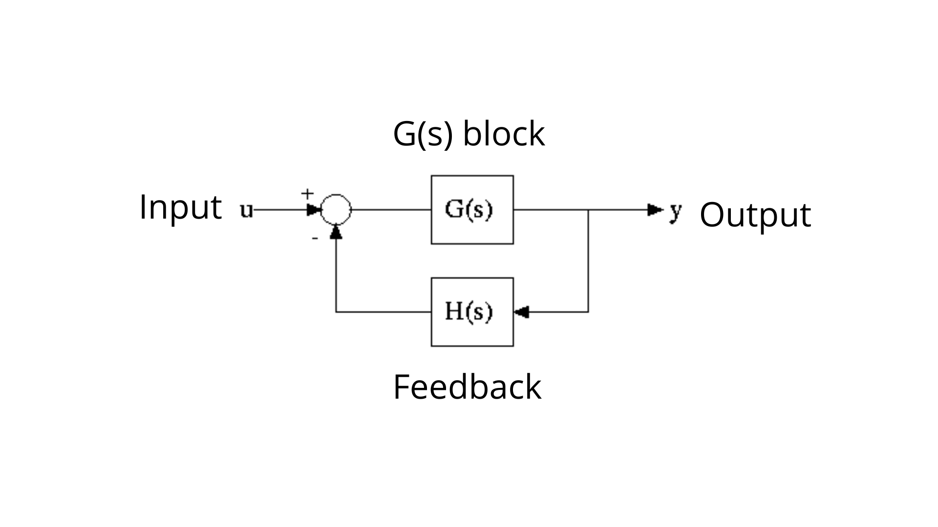
Control system block

Type of Systems:

The type of system is defined as the number of poles of the system present at the origin. It is an open-loop transfer system G(s)H(s) and should be a negative unity feedback system.

Type 0 System:

This is the type of system in which the open loop transfer function has no pole at the origin. For example,   is an example of Type 0 system.

Type 1 System:

This is the type of system in which the open loop transfer function has one pole at the origin. For example, is an example of Type 1 system.

Type 2 System:

This is the type of system in which the open loop transfer function has one pole at the origin. For example, is an example of Type 2 system.

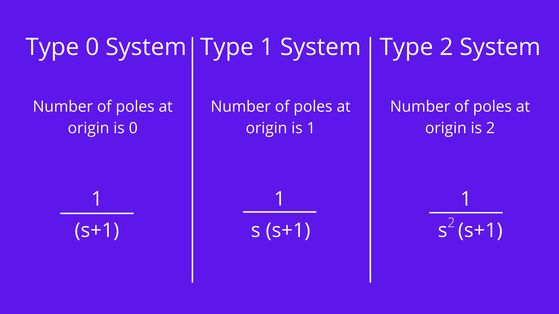
Types of system

The type of system is determined by the number of poles it has. If a system has an 'n' number of poles, it will be considered a Type 'n' system.

Root Locus:

Evans introduced the root locus technique in the control system in 1948. A physical system is represented by a transfer function in the form of:

We can find poles and zeroes from G(s). The location of poles and zeros is essential in keeping relative stability,  stability, and transient response and error analysis. When the system is put in working condition, stray inductance and capacitance get into the system, thus changing the location of poles and zeros. In the root locus technique in the control system, we will calculate the location of the roots, their locus of movement and other relevant information. This information will be used to comment on the system's performance.

Before introducing a root locus technique, it is essential to discuss a few of its benefits over other stability criteria. Some of the advantages of the root locus technique are written below:

Advantages of Root Locus Technique

• The root locus technique in the control system is easy to implement compared to other methods.
• With the help of the root locus, we can easily predict the whole system's performance.
• Root locus provides a better way to indicate the parameters.

Now, there are various terminologies related to the root locus technique that we will be using:

• Characteristic Equation Related to Root Locus Technique:  is known as the characteristic equation. If we differentiate the characteristic equation and equate , it is possible to obtain the necessary breakaway points.
• Break Away Points: Imagine if two root loci which start from a pole and move in the opposite direction collided with each other such that after the collision, they start symmetrically moving in different directions, and the breakaway points at which multiple roots of the characteristic equation occur, then the value of "k" is maximum at the points where the branches of root loci break away. Breakaway points may be accurate, imaginary or complex.
• Break-in Point: The condition of a break in to be there on the plot is written below: The root locus must be present between two adjacent zeros on the real axis.
• Centre of gravity: It is also known as the centroid of the system and the point on the plot, which indicates starting of the asymptotes. Mathematically, it is calculated by the difference in summation of poles and zeros in the transfer function when divided by the difference between the total number of poles and the total number of zeros. The Centre of gravity is always real, and it is denoted by

• Where N= number of poles
• M= number of zeroes
• Asymptotes of root loci: Asymptotes originate from the Centre of gravity or centroid and go to infinity at a definite angle. Asymptotes provide direction to the roof locus when they depart breakaway points.
• The angle of asymptotes: Asymptotes make some angle with the real axis, and this angle can be calculated from the formula:

Where p = 0, 1, 2…(N-M-1)

N is the total number of poles

M is the total number of zeroes

• The angle of arrival or departure: We calculate the angle of departure when complex poles exist in the system. The angle of departure can be calculated as 180-((sum of angles to a complex pole from the other poles)-(sum of angles to a complex pole from the zeros)).
• The intersection of Root Locus with the Imaginary Axis: To find the point of intersection between root locus with imaginary axis, we have to use the Routh Hurwitz criterion. First,  the auxiliary equation is found then the corresponding value of K will give the value of the point of intersection.
• Gain Margin: We define gain margin as a by which the design value of the gain factor can
• be multiplied before the system becomes unstable. Mathematically it is given by the formula:
• 
• Phase Margin: Phase margin is the magnitude of change needed in an open-loop system to make the closed-loop system unstable

The symmetry of root locus:

The root locus is symmetric about the x-axis or the real axis. How do we determine the value of K at any point on the root loci? Now there are generally two ways of determining the value of K, and each way is described below:

• Magnitude Criteria: At any points on root locus we can apply magnitude criteria as . By using this formula, we can find the value of K at any given point.
• Using Root Locus Plot: The value of "k" can be determined by:
• 

Root Locus Plot:

The root-locus technique in the control system is used to find the given system's stability. Now to find out the system's stability by using the root locus technique, we determine the range of values of "k" for which the system's overall performance will be satisfactory. In turn,  the operation is fully stable. There are some results that one should know to plot root locus. These results are written below:

• The region where the root locus exists: After plotting all the zeros and poles on the plane, we can
• find out the region of existence of the root locus by using one easy rule, which is written below. Only that segment will be considered in the making-root locus if the total number of poles and zeros at the right-hand side of the segment is odd.
• Calculating the number of separate root loci: A number of separate root loci is equal to the total number of roots if the number of roots is greater than the number of poles; otherwise, the number of separate root loci is equal to the total number of poles if the number of roots
• are greater than the number of zeros.

Plotting the root locus in MATLAB:

To plot the root locus in MATLAB, first, the transfer function needs to be initialised. There should be a numerator and a denominator of the respective system. Both the numerator and denominator will be a horizontal matrix, which will contain the coefficients of the numerator and denominator, respectively. Then the "tf(numerator, denominator)" function of the control system toolbox will be used so that the transfer function is ready.

The type of system depends upon the input of the numerator and the denominator. MATLAB has a function called "rlocfind()" for finding the root locus. It calculates and plots the root locus of a dynamic system when the feedback is from 0 to infinity.

After getting the root locus, we can use the "rlocfind()" function, which will enable us to click on a random area in the root locus plot, and then after clicking, we can get the value of "k" and the location of the poles.

The function "margin()" helps us find the phase margin, gain margin, phase crossover and gain crossover of the selected point.

Below are the respective outputs we have obtained using MATLAB for the different types of systems:  

Type 0 System:

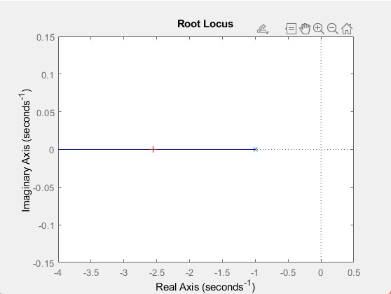
Type 0 plot

System Analysis is over. Here are the parameters:

 The value of k is:

    0.0020

 The location of closed-loop poles are:

   -1.0020

 The gain margin of the system is:

 The phase margin of the system is:

 The gain crossover of the system is:

 The phase crossover of the system is:

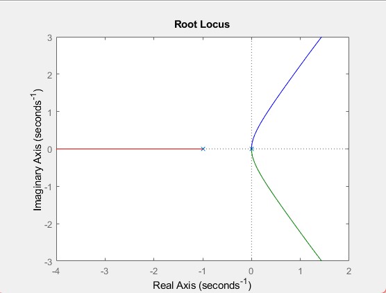
Type 1 System:

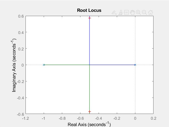
Type1 plot

System Analysis is over. Here are the parameters:

 The value of k is:

    0.3370

 The location of closed-loop poles are:

  -0.5000 + 0.2949i

  -0.5000 - 0.2949i

 The gain margin of the system is:

 The phase margin of the system is:

   51.8273

 The gain crossover of the system is:

 The phase crossover of the system is:

    0.7862

Type 2 system:

Type 2 plot

System Analysis is over. Here are the parameters:

 The value of k is:

    5.9399

 The location of closed-loop poles are:

  -2.2129 + 0.0000i

   0.6065 + 1.5220i

   0.6065 - 1.5220i

 The gain margin of the system is:

 The phase margin of the system is:

  -40.9750

 The gain crossover of the system is:

 The phase crossover of the system is:

    0.8685

MATLAB Code:

Conclusion:

In this blog, we have learned about a control system, the different types of systems, root loci, and some terminologies related to the root locus technique. Using the necessary functions in MATLAB, we have plotted the root locus for Type 0, Type 1 and Type 2 systems and found out different parameters of each type with the help of the Control System Toolbox.