Probability Tidbits 7 - All About Integration

As we discussed in tidbit 5, random variables are actually functions. These functions are non-negative everywhere and importantly measurable. This means for any measurable set in the output measurable space (typically (R,B)), the preimage of the measurable set must also be measurable in the input measurable space(arbitrary (Ω,F)). Since random variables preserve measurability of sets, it’s natural to integrate over some measurable real number domain (e.g. intervals) to assign a probability measure to it.

Recall in Riemann integration, we would approximate the integral of a function f:R→R by taking tall rectangles of fixed length but variable height and fitting it snugly under the function. Then, we’d take the limit as the fixed lengths go uniformly to 0 in order to get the precise area under the curve:

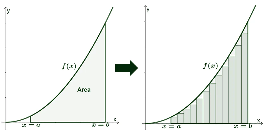
When it comes to measurable functions mapping from arbitrary (Ω,F) to the reals(instead of reals to reals), it makes sense to construct these rectangles a different way, the Lebesgue way.

Note that for the rest of this blog we’ll be using measurable functions to mean positive measurable functions. Too many words to type.

Simple Functions

When considering measurable functions that map Ω→R+, what is the simplest function you can think of that’s not just f(ω)=0∀ω∈Ω? Suppose we fix an arbitrary measurable set A∈F, then the indicator function of A is pretty simple:

1A(ω)={1 if ω∈A0 else

This map basically partitions the space of Ω into elements that are in A and those that aren’t. This function is obviously measurable, since A is measurable and Ac must be measurable since F is a σ-algebra. We can denote $\mu(1A) := \sum\Omega 1_A(\omega) = \mu(A),inthatwesummedupallelementsmeasuresinA$ with unit weights.

A function f is called simple if it can be constructed by a positive weighted sum of stepwise indicator functions of measurable sets A1,…,An (finite!) in F:

f(x)=n∑kak1Ak(x)

Subsequently,

μ(f)=n∑kakμ(Ak)

There are some obvious properties of simple functions. Let’s take f,g as simple functions and c∈R:

1. Almost everywhere equality: μ(f≠g)=0⟹μ(f)=μ(g).
2. Linearity: f+g is simple and cf is simple.
3. Monotonicity: f≤g⟹μ(f)≤μ(g)
4. Min/max: min(f,g) and max(f,g) are simple.
5. Composition: f composed with an indicator function 1A is simple.

Integrals of simple functions are also easy to reason about. Let’s start with a sequence of monotonically increasing simple functions hn such that the sequence converges to $1AforameasurablesetA \in \mathcal{F}.Is\text{lim}{n \to \infty} \mu(h_n) \to \mu(1_A)$? Or in other words, can we “pull out the limit”, so that:

μ(limn→∞hn)?=limn→∞μ(hn)

We can correspond these functions hn to measurable sets An:=ω:hn(ω)>1−ϵ for some ϵ (recall it’s also bounded above by the indicator functions). Note that (1−ϵ)μ(An)≤μ(hn) by definition, since it’s only a subset of the outcomes for hn:

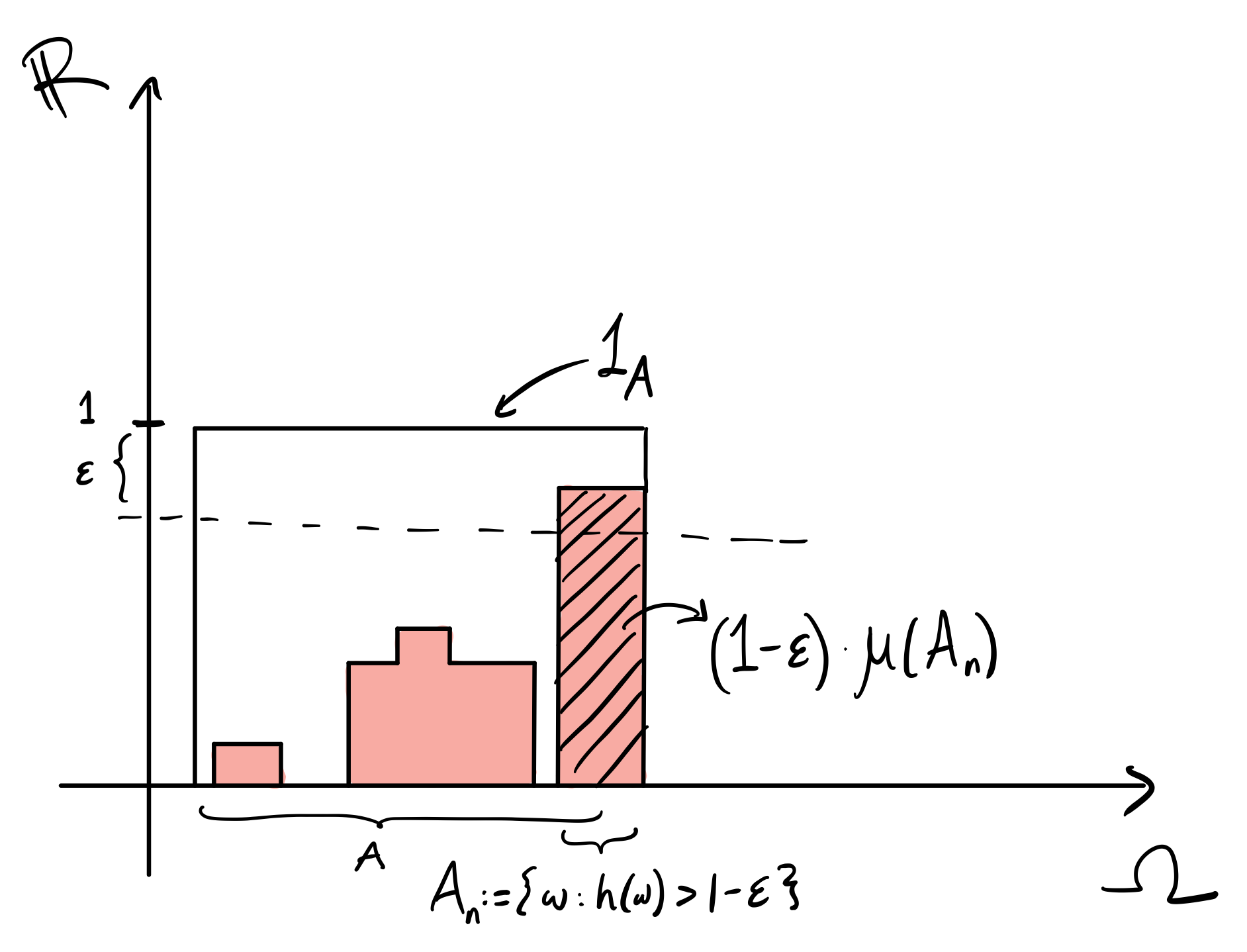
The sequence of sets An converge to A since $h_n \to 1AandA = {\omega: 1_A(\omega) = 1 > 1-\epsilon}.Thismeans\lim{n \to \infty} \mu(h_n) \geq (1-\epsilon)\mu(A).Nowwetake\epsilonsmallandwehavethat\lim_{n \to \infty} \mu(h_n) = \mu(A) = \mu(\lim_{n \to \infty} h_n) = \mu(1_A)$. Note that we started with a simple indicator function in the above example, but it can be pretty trivially extended to any simple function.

Measurable functions aren’t always simple. For an arbitary measurable f:Ω→R+ we can’t just represent it with a finite sum of indicator functions. Just like how we take the limit as the rectangles widths go to zero in the Riemann integral, we can take a limit on a sequence of monotonically increasing simple functions bounded by f. The integral of f can thus be expressed as the integral of the least upper bound of these simple functions:

μ(f):=sup{μ(h):h is a simple function,h≤f}

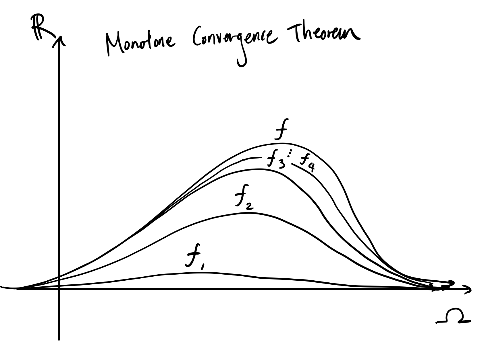
Monotone Convergence Theorem

This theorem is basically the entire foundation of lebesgue integration. Just like how we built up integral approximations of continuous functions using rectangles, monotone convergence theorem tells us we can define the lebesgue integral using approximations of measurable functions using simple functions. Specifically, it states for a sequence (fn) of monotonically increasing measurable functions which converge pointwise to some function f, f is measurable and the lebesgue integral also converges:

limn→∞μ(fn)=μ(limn→∞fn):=μ(f)

First, let’s fix ϵ>0 and some simple function 0≤h≤f. The set

An:={ω:fn(ω)≥(1−ϵ)h(ω)} is interesting (note that this is slightly different than the simple function case, since we’re using ≥ here). As n→∞, An→Ω since fn will eventually converge to f≥h. We know that $\mu(f_n) \geq \mu(f_n 1{A_n}),sincewe′rerestrictingourdomaintoasmallersetA_n.Wealsoknowthat\mu(f_n 1{A_n}) \geq \mu((1-\epsilon)h 1_{A_n})$. Now we have a chain of inequalities which we can take the limit of:

μ(fn)≥μ(fn1An)≥μ((1−ϵ)h1An)⟹limn→∞μ(fn)≥limn→∞μ(fn1An)≥limn→∞μ((1−ϵ)h1An) Note that since h1An and h1A are simple, from previous results on simple functions we have:

limn→∞μ((1−ϵ)h1An)=μ(limn→∞(1−ϵ)h1An)=(1−ϵ)μ(h)

Since An→Ω. Since we took an arbitrary ϵ, we can say that:

limn→∞μ(fn)≥μ(h)

And since we took an arbitrary simple h, we can say that:

limn→∞μ(fn)≥suph≤fμ(h):=μ(f)=μ(limn→∞fn)

by definition of the lebesgue integral on measurable f, so we’re done! Here’s an picture on what the fn’s may look like:

You might be saying right now:

So what? Big deal you moved the limit from inside to outside. Why do we care?

Let me convince you this is a big deal, by using this theorem to trivially prove some other lemmas and theorems in integration theory which we’ll be using as hammers to problems in the future.

Fatou’s Lemma

We can easily prove Fatou’s Lemma (and its reverse counterpart) with monotone convergence theorem. The lemmas are useful to reason about bounds of a sequence of measurable functions which may not necessarily be monotonically increasing or decreasing. Specifically, the lemmas state that for a sequence of measurable functions (fn):

μ(lim infnfn)≤lim infnμ(fn)(Fatou's Lemma)μ(lim supnfn)≥lim infnμ(fn)(Reverse Fatou's Lemma)μ(lim infnfn)≤lim infnμ(fn)≤lim infnμ(fn)≤μ(lim supnfn)(Fatou-Lebesgue Theorem)

Here, we just have to look at gk:=infn≥kfn which is an increasing sequence of functions on k, converging to some function gk↑g. We know that:

gn≤fn∀n⟹μ(gn)≤μ(fn)∀n⟹μ(gn)≤infk≥nμ(fk)⟹limnμ(gn)∗=μ(limngn)=μ(lim infnfn)≤limninfk≥nμ(fk)=lim infnμ(fn)

In the result, the equality with a star on top is where we applied monotone convergence theorem and the rest were just by definition. You can essentially use the same approach to prove reverse Fatou’s lemma. The theorem follows pretty obviously.

Dominated Convergence Theorem

Dominated convergence theorem essentially says that if a sequence of measurable functions fn which converge to f is bounded by a nice function g, then f must also be nice. Here, we define niceness as μ-integrable. For some measure space (Ω,F,μ) if a function f is μ-measurable it is denoted f∈L1(Ω,F,μ) if:

|μ(f)|≤μ(|f|)<∞

where the first inequality is just due to Holder’s inequality.

So back to the theorem. It states that (fn) is dominated by g∈L1(Ω,F,μ) if:

|fn(x)|≤g(x)∀fn,x

If this holds, then f∈L1(Ω,F,μ), and μ(fn)↑μ(f)(we can pull out the limit) . We know by triangle inequality $

f_n - f

< 2g \implies h_n := 2g -

f_n - f

,i.e.(h_n)isasequenceofpositivemeasurablefunctions.Wecanprovethat\mu(

f_n - f

)$ vanishes:

μ(2g)=μ(lim infnhn)∗≤lim infnμ(hn)=μ(2g)−lim supnμ(|fn−f|)⟹0≤lim infnμ(|fn−f|)∗≤lim supnμ(|fn−f|)≤0⟹limnμ(|fn−f|)→0

where the starred inequality is due to Fatou’s lemmas.

Counterexamples to Dominated Convergence Theorem

Say we don’t have a dominating function g for a sequence of functions (fn). Then it’s hard to say whether we can pull out the limit. Suppose we have the function fn(x)=1x∗1[1n,1). μ(fn)<∞∀n, but the limit is the integral of log(1)−log(0)=∞. Here we couldn’t bound fn by any dominating function in L1(Ω,F,μ).

Another canonical example is the function fn(x)=n∗1(0,1n]. This function converges to the zero function so μ(limfn)=0, but μ(fn)=1∀n⟹limμ(fn)=1. This is another case of us unable to bound fn(x) by any dominating function.