Many organizations are discovering the tremendous value that graph databases provide in solving complex problems on connected data. Where relational databases focus on the data in the data model, they struggle to derive value from the relationships between data items in the same data model. Graph databases are designed to derive value from both the data and the relationships in your data model.

What happens when the graph data you need to capture and analyze has a geographic element? What happens when much of your analysis becomes concerned with the “where” aspect of your data model?

The Uber Engineering team has developed the Hierarchical Hexagonal Index called H3 as a model for dividing the world up into hexagons, and they’ve created a set of APIs that are used to interact with those hexagons. What they didn’t provide is a database or storage model for H3 APIs. That’s where InfiniteGraph comes in.

This article describes our approach to implementing a graph data model to represent the Uber H3 index. Our model extends the H3 model by allowing you to associate your domain data model components to the H3 hexagons stored in the database.

All of this comes together to give you a powerful set of capabilities to store and query your domain data in terms of your domain model and in terms of the underlying H3 geographic model. By using InfiniteGraph as the graph database platform, complex queries can be performed on this data in near real-time at massive speed and scale for high-performance systems and analysis. InfiniteGraph supports both vertical and horizontal scalability as well as scalability through distribution so you can easily scale your application up and down.

A Unified Geographic Context: A Story

In order to develop a deeper understanding of their existing operations and help them plan for the future, a national retailer collects data from a wide variety of sources across all of their stores. All of the collected data provides visibility into things that have a direct impact on their business.

The retailer collects data on:

• Purchase:
  • What was purchased
  • When it was purchased
  • Where it was purchased
• Customer:
  • Where the customer lives
  • The customer’s email, phone number, and purchase history
• Supply chain:
  • Which companies supply which items
  • Delivery delays
  • Wholesale price fluctuations
• Operational store data:
  • Labor costs
  • Utility costs
  • Inventory losses
• Weather:
  • Daily temperatures
  • Impending storms

Every data item is stored on a digital map creating a unified geographic context. Purchase information is associated with the map location of the store where the purchase was made. Customer data is associated with the home address, neighborhood, and community of each customer.  Supply chain data is associated with the locations of the suppliers and the delivery routes they use. Operational store data is associated with the locations of the store. And finally, weather data is applied to the map for all of the regions that pertain to stores, customers, and the supply chain.

When using a graph database, all of this data comes together to provide a powerful new tool that allows the retailer to preform predictive analytics on customer buying patterns and demographics, complex supply chain interactions, and the impact of severe weather on both sales and supply chain performance. 

What Is a Graph Database?

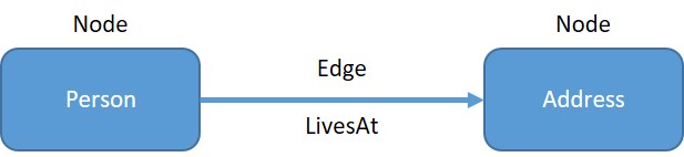
Fundamentally, a graph database is a database that represents data as nodes and edges. Nodes typically represent data items from your domain (like Person, Place, or Thing) and edges represent the relationships between the nodes. For example, we might represent a person and an address as nodes and we might then create an edge between them to represent a “LivesAt” relationship.

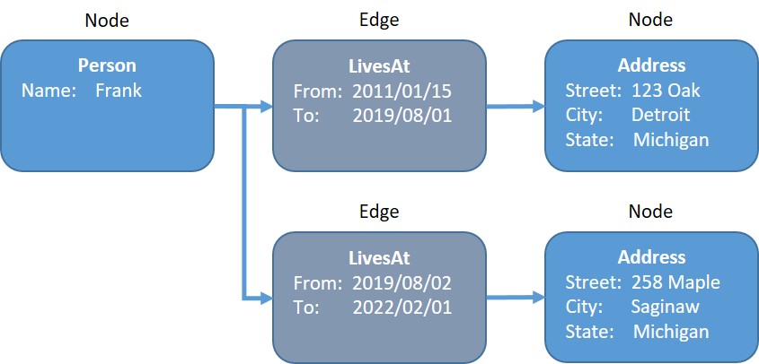
The graph data model provides great flexibility for representing data. We can expand on our Person-LivesAt-Address model by including a date range in the LivesAt edge so that we can represent all of the places a person has lived.

What Is InfiniteGraph?

InfiniteGraph is an object-oriented graph database platform. InfiniteGraph uses a federated architecture to achieve massive scalability. A single InfiniteGraph federated database can be distributed across 65,000 servers and can hold a theoretical limit of 1.84 x 1019 objects.

Developers create applications that use the InfiniteGraph API libraries to interact with federated databases. InfiniteGraph is deployed with two lightweight servers: a lock server that coordinates locks across all running applications, and a page server that responds to page requests from the InfiniteGraph API running in client applications. All graph processing happens in the client application and the API. The API serves as the database server which linked into the client application, making it incredibly fast.

Where many other graph database products use a property model approach, InfiniteGraph uses a schema-based approach. InfiniteGraph’s schema-based approach requires that developers create schema definitions for the data types they will be storing before they store any data. This provides a number of advantages including support for InfiniteGraph’s Placement Management Capability (PMC). The PMC is a rules-based system that allows developers to define rules that dictate how data is placed in the database. PMC rules can tell InfiniteGraph that two objects that might be of different types (Person and Address, for example) should be placed on the same disk page because they will frequently be used together.

When a user performs a query for a Person, they are likely to next ask for the related Address object. If those two objects are on the same disk page, when the disk page is read in response to the query for the Person object, the related Address object on the same disk page will be read into the InfiniteGraph page cache in the client application. When the user then asks for the Address object, a second-page read will not be required because the page with the Address object is already in memory.

All of these capabilities come together to create a massively scalable, high-performance object-graph analytics platform upon which customers can build cutting-edge applications.

What Is H3?

H3 is Uber’s hexagonal hierarchical spatial indexing system.

“…Uber developed our grid system for efficiently optimizing ride pricing and dispatch, for visualizing and exploring spatial data. H3 enables us to analyze geographic information to set dynamic prices and make other decisions on a city-wide level. We use H3 as the grid system for analysis and optimization throughout our marketplaces. H3 was designed for this purpose, and led us to make some choices such as using hexagonal, hierarchical indexes.”
(Uber Engineering, 2022)

H3 Hexagon Addresses

H3 assigns a unique address to every hexagon. H3 Addresses are hexadecimal values of the form “852a1077fffffff” and they represent a specific hexagon.

The address allows H3 to determine:

• The hexagon’s resolution
• The latitude and longitude of the center of the hexagon
• The latitude and longitude of each of the corners of the hexagon
• Its parent address (assuming it’s not a resolution 0 hexagon)
• The H3 addresses of its seven children (assuming it’s not a resolution 15 hexagon)

The H3 address is primarily how you interact with the H3 indexing system.

H3 Resolutions

H3 also introduces the concept of resolutions to support layers of hexagons of different sizes. The details for each resolution are given in the table below. At every resolution except 15, every hexagon has seven children. Each child hexagon covers approximately 1/7 of the area covered by the child’s parent hexagon. At every resolution except 0, every hexagon has one parent. Each parent hexagon covers approximately 7 times the area covered by the child. Figure 1 shows a single hexagon at resolution 9, its seven children at resolution 10, and those hexagon’s children at resolution 11.

Figure 1: H3 Hexagon Resolutions

Building an H3 Graph Database

The H3 APIs support a wide range of conversions that make H3 an elegant tool for managing geographical data models. However, H3 does not provide a storage model. H3 does not come with an underlying database. It is essentially a set of tools for deriving information about hexagons mapped onto planet Earth.

Because H3 gives us interesting capabilities like computing the address of a hexagon given its latitude/longitude or giving us the addresses of a hexagon’s neighbors, it seems reasonable to create a graph database of H3 hexagon objects where each hexagon is a node and it is edge-connected to its neighbors, its parent (resolution minus one), and its children (resolution plus one).

That is exactly what we’ve done.

An InfiniteGraph Schema for H3 Data

The initial schema for a Hexagon class is pretty straightforward. We need an address, the resolution, a reference to the parent Hexagon, a list of references to child Hexagons, and a list of references to neighbor Hexagons.

That gives us the following:

This is a great start, but in order to be useful, we need to add a few more things. First, in order to support a wider range of geographic queries, we need to add fields that give us the minimums and maximums for the latitude and longitude of the hexagon. Finally, we’d like to associate some data with our Hexagon objects so we’ll need a reference to some kind of data object that we’ll call HexagonData for now.

That gives us the following definition:

This gives us a powerful foundation upon which we can build an H3 graph database.

The HexagonData Class

Having a graph database of edge-connected hexagons is great. It gives us the ability to perform graph navigational queries across the connected hexagons. However, it’s not very useful until we can qualify our navigational queries using some kind of domain data that we’ve associated with the hexagons.

One approach would be to put the domain data attributes in the Hexagon class definition. A better approach would be to separate our Hexagon objects from our domain data. That’s where the HexagonData class comes into play.

The HexagonData class, shown below, has a single attribute, “itemMap”. The itemMap attribute is a NameToReferenceMap which allows us to map a string key to reference to a DataItem object where an actual data value will be stored. In this case, the key is essentially the data field name, and the associated field value is contained in the referenced DataItem object.

The HexagonData object serves as a level of indirection between the Hexagon map objects and any data that might be associated with them. It is probably safe to assume that the Hexagon object won’t change very often after its initial creation. It is probably also safe to assume that there could likely be a large volume of data being ingested and associated with each Hexagon, or more specifically, with each HexagonData object.

Another advantage of separating the Hexagon objects from the HexagonData and DataItem object is object placement. We can place the Hexagon objects in one part of the federation and then put the HexagonData and DataItem objects in a completely different part of the federation. A good Placement strategy will minimize lock contention in an environment where hundreds or even thousands of threads are reading from and writing to the database.

The DataItem Class

The DataItem class is the last stop on our journey for actually associating a value with a Hexagon.

This is a simplified version of the DataItem class:

The DataItem class has a timestamp used to indicate when the value came into existence and then a strValue String attribute to store text data and a realValue to store a decimal value. In the current design, there is nothing in the DataItem object that indicates what the value represents. That information is derived from the key in the itemMap in the HexagonData object that pointed to the DataItem object.

A Picture Is Worth a Thousand Words…

Given a particular Hexagon object, the “path” to the DataItems associated with it is shown below.

In this diagram, there is some Hexagon represented by the variable “$hex.” It has an attribute “data” that is a reference to a HexagonData object. That HexagonData object has an attribute: “itemMap.” The itemMap has a key-value pair with a key of “Population.density” that is associated with a reference to a DataItem object where the value for the Population.density for the Hexagon, $hex, is stored. The same HexagonData object also has a key, “Climate.avgTemp,” that is associated with a DataItem where the value for Climate.avgTemp is stored.

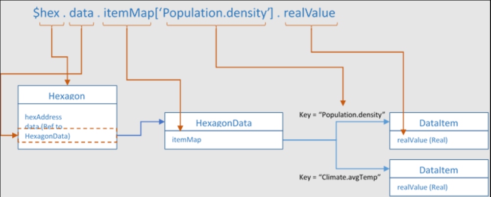
Figure 2: Path to DataItems

Queries

InfiniteGraph supports several different kinds of queries that fall into two general categories: FROM queries and MATCH queries.

FROM Queries

FROM queries allow us to return data from an object based on a particular class type and possibly a predicate. For example, the following query returns every attribute from all Hexagon objects:

If we only wanted the address attribute of all Hexagon objects, we could modify the return clause to only return the address:

We can add a predicate to narrow our result set.

Finally, we can use the dot-notation to return the DataItem objects connected to every Hexagon object that meets our WHERE clause.

MATCH Queries

Match queries are where we can really harness the power of the graph.

A simple MATCH query allows us to find all of the paths to our degree-1 neighbors:

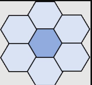
Figure 3: Degree-1 Neighbors

If we didn’t want the paths but instead wanted the addresses in out degree = 1 neighbors, we could get that by modifying what we return from “p” to “h2.addresses.”

Here, we’ve assigned a variable, h2, to the target hexagon and the returned h2.address. This will give us a list of the zero to six addresses of the degree=1 neighboring Hexagon objects.

If we wanted to get the addresses of the degree=2 neighboring Hexagons, we would simply add another edge-node clause in the middle of our query:

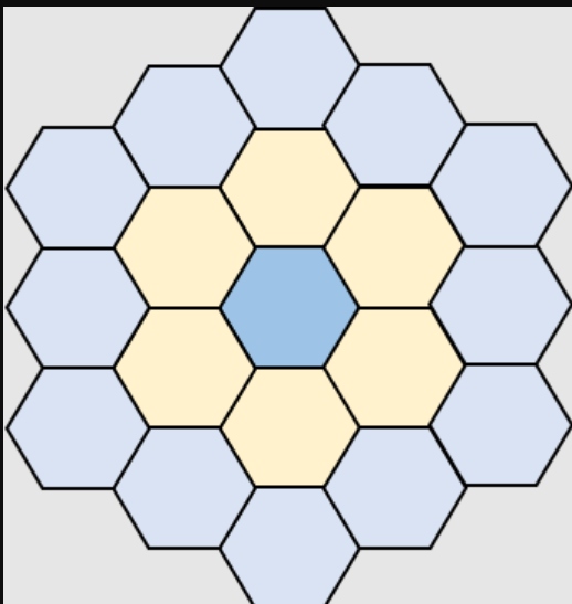
Figure 4: Degree-2 Neighbors

Path-Between Queries

We can use the MATCH Query to find the paths between two Hexagon objects. In the case of our Hexagon grid system, there will be many paths so we are really only interested in the shortest path between two Hexagons. Note that it is also important to set an upper bound on how far out we want the query to search, otherwise the query may end up taking a very long time to run because of the volume of data that will need to be processed to find the endpoint. This is done by setting a variable but bounded edge qualifier such as “-[:neighbors *1..20]->”. The “*1..20” says to get from 1 to no more than 20 hops out when conducting the search.

Given two Hexagon addresses we can find the shortest path between them by incorporating the SHORTEST operator into our MATCH query as follows:

This is the simplest form of a path-between query.

Data-Qualified MATCH Queries

Suppose we were given a Hexagon and we were asked to find the nearest Hexagon with an average temperature of greater than 72 degrees within some property within 20 degrees. It’s easy enough to do by simply adding a qualifier to the target Hexagon.

This query will find the shortest path to a neighboring Hexagon within 20 degrees where the “Climate.avgTemp” value is greater than 72.0 degrees.

Qualifying Hexagons Along the Path

The last query demonstrated how to qualify the vertex Hexagon at the end of a path. What if we wanted to qualify all of the hexagons along a path; specifically, what if we wanted to find a path from one Hexagon to another Hexagon where every Hexagon along the path met some criteria? For this, we will take a slightly different approach and use the DO Language Weighted Graph Weight Calculator operator.

The weight calculator allows you to define a set of functions to calculate the weight of an edge based on some criteria. If you had a graph of cities connected by roads, you might say the roads were edges between the city vertices and that the weight of each edge is the length of each road.

Figure 5: Weighted Edges

We can expand upon the concepts of weighted graphs and queries and the dot notation that we talked about earlier to find the shortest path between two Hexagons where each Hexagon along the path meets some criteria. In this example, we want to find a Hexagon path from a defined origin Hexagon to a defined target Hexagon where every Hexagon along the path has a Climate.avgTemp greater than 72.0 degrees.

In our Hexagon class definition, the “neighbors” edges do not have attributes. That’s fine. We will infer an edge weight by examining the Hexagon on the far side of each neighbor's edge reference.

We want every edge that leads to a Hexagon that meets our criteria to have a low edge weight and conversely, we want every edge that leads to a Hexagon that does not meet our criteria to have a very high edge weight. Here is how we do that using a WEIGHT CALCULATOR:

This weight calculator defines two edge-matching patterns. The first one matches edges that originate on a Hexagon and lead to a Hexagon where the Climate.avgTemp is > 72.00. For edges that match these criteria, the weight calculator will assign a weight of 1.

The second edge-matching pattern will match edges that originate on a Hexagon and lead to a Hexagon where the Climate.avgTemp is <= 72.00. To any edge that matches this pattern, we will assign a weight of 1000.

Using this WEIGHT CALCULATOR, our query then becomes:

This query will return the lightest weight path (shortest because qualifying edges have a weight of one) and will disqualify any path whose weight (length) is over 21.0, thus returning a resulting path if one exists.

The real beauty of the WEIGHT CALCULATOR is that we can change it or even write new ones to qualify edges on the same graph data without having to change the data on the nodes and edge. The WEIGHT CALCULATOR is dynamic and computes weights on the fly from any available node and edge data that are accessible to the from-node, the edge, or the to-node. In our case, we created two edge weight functions that used information in objects connected to the to-node.

Conclusion

The H3 Hierarchical Hexagon Indexing scheme is a brilliant way to organize, manage, and interact with geographic data. Creating an InfiniteGraph graph database hexagon model provides an amazing foundation upon which you can capture other data and associate it with the hexagons. This all leads to a geographic graph analytics platform that can be used to perform advanced and complex data analytics on massive volumes of data.