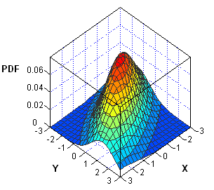
I've been working on a new book about Simulating Data with SAS. In researching the chapter on simulation of multivariate data, I've noticed that the probability density function (PDF) of multivariate distributions is often specified in a matrix form. Consequently, the multivariate density can usually be computed by using the SAS/IML matrix language. As an example, this article describes how to compute the multivariate normal probability density for an arbitrary number of variables.

Compute the multivariate normal PDF

The density for the multivariate distribution centered at μ with covariance Σ is given by the following formula, which I copied from a Wikipedia article:

The argument to the EXP function involves the expression d2=(x-μ)TΣ-1(x-μ), where d is the Mahalanobis distance between the multidimensional point x and the mean vector μ. I have previous written a SAS/IML function that computes the Mahalanobis distance in SAS, so it is simple to construct a SAS/IML function that computes the multivariate normal PDF for any dimension:

proc iml;
/* Cut and paste the definition of the Mahalanobis module. See
https://blogs.sas.com/content/iml/2012/02/22/how-to-compute-mahalanobis-distance-in-sas/ */
start MVNormalPDF(x, mu, cov);
   p = nrow(cov);
   const = (2*constant("PI"))##(p/2) * sqrt(det(cov));
   d = Mahalanobis(x, mu, cov);
   phi = exp( -0.5*d#d ) / const;
   return( phi );
finish;

The MVNormalPDF function is essentially an implementation of the PDF formula, except that the (efficient) Mahalanobis function is used instead of explicitly forming the expression (x-μ)TΣ-1(x-μ). Incidentally, the formula assumes that x and μ are a column vectors. However, the Mahalanobis and MVNormalPDF functions assume that mu is a row vector, and evaluates the PDF on each row of the x matrix.

Evaluating the multivariate normal PDF

Although it is not apparent at first glance, the MVNormalPDF function is vectorized, which means that the x argument can be an N x p matrix that represents N different p-dimensional points. The vectorization results from the fact that the Mahalanobis function is vectorized.

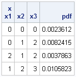
This means that you can evaluate the PDF at many points by using a single call, as shown below for a three-dimensional example:

Mu  = {1 2 3};
Cov = {3 2 1, 
       2 4 0,
       1 0 5};
x = {0 0 0,
     0 1 2,
     2 1 2,
     1 2 3};
pdf = MVNormalPDF(x, Mu, Cov);
print x[c=("x1":"x3")] pdf;

Visualize the bivariate normal PDF

In the case of two variables, you can visualize the bivariate normal density by creating a surface plot or contour plot. In either case, you need to evaluate the MVNormalPDF function at a grid of (x,y) values. You can use the Define2DGrid function to generate evenly spaced (x,y) values on a uniform grid. The following SAS/IML statements load the Define2DGrid function, evaluate the bivariate normal density at a grid of points, and write the data to a SAS data set:

/* define or load Define2DGrid module:
https://blogs.sas.com/content/iml/2011/01/21/how-to-create-a-grid-of-values/ */
load module=Define2DGrid;
Mu = {0 0};
Cov = {4 2, /* correlation coefficient is sqrt(2) */
       2 2};
x = Define2DGrid( -3, 3, 31, -3, 3, 31 ); /* grid is [-3,3]x[-3,3] */
density = MVNormalPDF(x, Mu, Cov);
 
x1 = x[,1]; x2 = x[,2];
create BivarDensity var {"x1" "x2" "Density"};
append;
close BivarDensity;
quit;

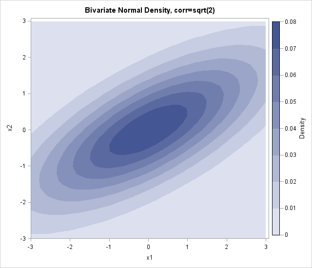
Earlier this week, I showed how to create a contour plot in SAS by using the Graph Template Language (GTL). Assuming that the ContourPlotParm template has been defined, the following call to the SGRENDER procedure creates a contour plot of the bivariate normal data:

proc sgrender data=BivarDensity template=ContourPlotParm;
dynamic _TITLE="Bivariate Normal Density, corr=sqrt(2) "
        _X="x1" _Y="x2" _Z="Density";
run;