Reunderstanding The Mathematics Behind Principal Component Analysis

As we all know, Principal Component Analysis (PCA) is a dimensionality reduction algorithm that can be used to significantly speed up your unsupervised feature learning algorithm. Most of us just know the procedure of PCA. In other words, we know how to use the algorithm but do not know how it comes. In this post, I summarize the procedure and mathematics of PCA based on materials of reference.

Procedure of PCA

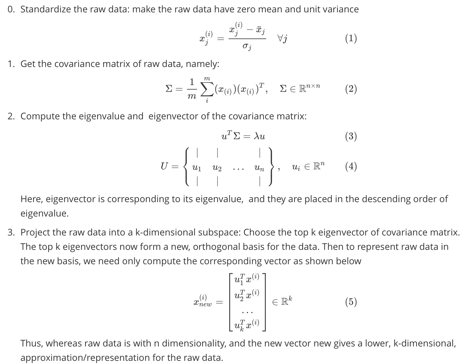
Suppose we have a dataset x(1),x(2),…,x(m)x(1),x(2),…,x(m) with n dimension inputs. We want to reduce the data from nn dimension to kk dimension (k<<n)(k<<n) using PCA. The procedure of PCA is shown below (Owing to the mathematical formual rendering problem, I use picture to display the procedure):

Mathematics behind PCA

In the previous section, I present the procedure of PCA. What a simple algorithm it looks like. However, do we actually know why we calculate the eigenvector of covariance matrix, getting the basis of new subspace.

The motivation of PCA is remaining as much information of raw data as possible by projecting raw data into lower subspace. In other words, we hope remain as much variance of raw data as possible in the new space.

In the formula (5), we see the projection of raw data. The length (variance) of the projection of xx onto uu is given by xTuxTu. I.e., if x(i)x(i) is a point in the dataset, then its projection onto uu is distance xTuxTu from the origin. Hence to maximize the variance, we can formulate it as an optimization problem:

This is a maximization problem with constraint. It can be reformulated as:

To get the (local) optimum of the constrained problem, we use the method of Lagrange multipliers:

Note that λλ is the Lagrange multipliers not the eigenvalue of covariance matrix. Now let us take the partial derivatives of formula (10) with respect to uu and λλ. Then let the derivatives equal to zero:

We can see that the formula (11) is equivalent to formula (3). Thus choosing the new basis of lower space is equivalent to getting the top-k eigenvector of covariance matrix of raw data.

See! The dimensionality reduction problem is intrinsically a constrained maximization problem. We use the method of Lagrangian multiplier to solve the problem.

Reference

http://59.80.44.100/cs229.stanford.edu/notes/cs229-notes10.pdf

http://ufldl.stanford.edu/wiki/index.php/PCA