Operating Systems

CPU Scheduling

References:

1. Abraham Silberschatz, Greg Gagne, and Peter Baer Galvin, "Operating System Concepts, Ninth Edition ", Chapter 6

6.1 Basic Concepts

• Almost all programs have some alternating cycle of CPU number crunching and waiting for I/O of some kind. ( Even a simple fetch from memory takes a long time relative to CPU speeds. )
• In a simple system running a single process, the time spent waiting for I/O is wasted, and those CPU cycles are lost forever.
• A scheduling system allows one process to use the CPU while another is waiting for I/O, thereby making full use of otherwise lost CPU cycles.
• The challenge is to make the overall system as "efficient" and "fair" as possible, subject to varying and often dynamic conditions, and where "efficient" and "fair" are somewhat subjective terms, often subject to shifting priority policies.

6.1.1 CPU-I/O Burst Cycle

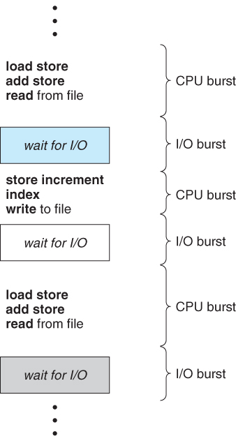
• Almost all processes alternate between two states in a continuing cycle, as shown in Figure 6.1 below :
  • A CPU burst of performing calculations, and
  • An I/O burst, waiting for data transfer in or out of the system.

Figure 6.1 - Alternating sequence of CPU and I/O bursts.

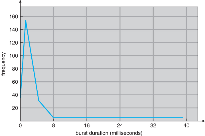
• CPU bursts vary from process to process, and from program to program, but an extensive study shows frequency patterns similar to that shown in Figure 6.2:

Figure 6.2 - Histogram of CPU-burst durations.

6.1.2 CPU Scheduler

• Whenever the CPU becomes idle, it is the job of the CPU Scheduler ( a.k.a. the short-term scheduler ) to select another process from the ready queue to run next.
• The storage structure for the ready queue and the algorithm used to select the next process are not necessarily a FIFO queue. There are several alternatives to choose from, as well as numerous adjustable parameters for each algorithm, which is the basic subject of this entire chapter.

6.1.3. Preemptive Scheduling

• CPU scheduling decisions take place under one of four conditions:
  1. When a process switches from the running state to the waiting state, such as for an I/O request or invocation of the wait( ) system call.
  2. When a process switches from the running state to the ready state, for example in response to an interrupt.
  3. When a process switches from the waiting state to the ready state, say at completion of I/O or a return from wait( ).
  4. When a process terminates.
• For conditions 1 and 4 there is no choice - A new process must be selected.
• For conditions 2 and 3 there is a choice - To either continue running the current process, or select a different one.
• If scheduling takes place only under conditions 1 and 4, the system is said to be non-preemptive, or cooperative. Under these conditions, once a process starts running it keeps running, until it either voluntarily blocks or until it finishes. Otherwise the system is said to be preemptive.
• Windows used non-preemptive scheduling up to Windows 3.x, and started using pre-emptive scheduling with Win95. Macs used non-preemptive prior to OSX, and pre-emptive since then. Note that pre-emptive scheduling is only possible on hardware that supports a timer interrupt.
• Note that pre-emptive scheduling can cause problems when two processes share data, because one process may get interrupted in the middle of updating shared data structures. Chapter 5 examined this issue in greater detail.
• Preemption can also be a problem if the kernel is busy implementing a system call ( e.g. updating critical kernel data structures ) when the preemption occurs. Most modern UNIXes deal with this problem by making the process wait until the system call has either completed or blocked before allowing the preemption Unfortunately this solution is problematic for real-time systems, as real-time response can no longer be guaranteed.
• Some critical sections of code protect themselves from con currency problems by disabling interrupts before entering the critical section and re-enabling interrupts on exiting the section. Needless to say, this should only be done in rare situations, and only on very short pieces of code that will finish quickly, ( usually just a few machine instructions. )

6.1.4 Dispatcher

• The dispatcher is the module that gives control of the CPU to the process selected by the scheduler. This function involves:
  • Switching context.
  • Switching to user mode.
  • Jumping to the proper location in the newly loaded program.
• The dispatcher needs to be as fast as possible, as it is run on every context switch. The time consumed by the dispatcher is known as dispatch latency.

6.2 Scheduling Criteria

• There are several different criteria to consider when trying to select the "best" scheduling algorithm for a particular situation and environment, including:
  • CPU utilization - Ideally the CPU would be busy 100% of the time, so as to waste 0 CPU cycles. On a real system CPU usage should range from 40% ( lightly loaded ) to 90% ( heavily loaded. )
  • Throughput - Number of processes completed per unit time. May range from 10 / second to 1 / hour depending on the specific processes.
  • Turnaround time - Time required for a particular process to complete, from submission time to completion. ( Wall clock time. )
  • Waiting time - How much time processes spend in the ready queue waiting their turn to get on the CPU.
    • ( Load average - The average number of processes sitting in the ready queue waiting their turn to get into the CPU. Reported in 1-minute, 5-minute, and 15-minute averages by "uptime" and "who". )
  • Response time - The time taken in an interactive program from the issuance of a command to the commence of a response to that command.
• In general one wants to optimize the average value of a criteria ( Maximize CPU utilization and throughput, and minimize all the others. ) However some times one wants to do something different, such as to minimize the maximum response time.
• Sometimes it is most desirable to minimize the variance of a criteria than the actual value. I.e. users are more accepting of a consistent predictable system than an inconsistent one, even if it is a little bit slower.

6.3 Scheduling Algorithms

The following subsections will explain several common scheduling strategies, looking at only a single CPU burst each for a small number of processes. Obviously real systems have to deal with a lot more simultaneous processes executing their CPU-I/O burst cycles.

6.3.1 First-Come First-Serve Scheduling, FCFS

• FCFS is very simple - Just a FIFO queue, like customers waiting in line at the bank or the post office or at a copying machine.
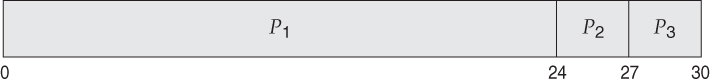
• Unfortunately, however, FCFS can yield some very long average wait times, particularly if the first process to get there takes a long time. For example, consider the following three processes:

Process Burst Time

• In the first Gantt chart below, process P1 arrives first. The average waiting time for the three processes is ( 0 + 24 + 27 ) / 3 = 17.0 ms.
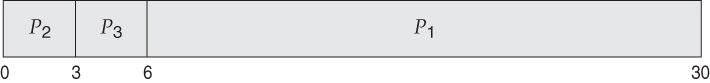
• In the second Gantt chart below, the same three processes have an average wait time of ( 0 + 3 + 6 ) / 3 = 3.0 ms. The total run time for the three bursts is the same, but in the second case two of the three finish much quicker, and the other process is only delayed by a short amount.

• FCFS can also block the system in a busy dynamic system in another way, known as the convoy effect. When one CPU intensive process blocks the CPU, a number of I/O intensive processes can get backed up behind it, leaving the I/O devices idle. When the CPU hog finally relinquishes the CPU, then the I/O processes pass through the CPU quickly, leaving the CPU idle while everyone queues up for I/O, and then the cycle repeats itself when the CPU intensive process gets back to the ready queue.

6.3.2 Shortest-Job-First Scheduling, SJF

• The idea behind the SJF algorithm is to pick the quickest fastest little job that needs to be done, get it out of the way first, and then pick the next smallest fastest job to do next.
• ( Technically this algorithm picks a process based on the next shortest CPU burst, not the overall process time. )
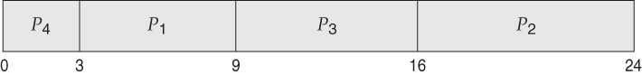
• For example, the Gantt chart below is based upon the following CPU burst times, ( and the assumption that all jobs arrive at the same time. )

Process Burst Time

• In the case above the average wait time is ( 0 + 3 + 9 + 16 ) / 4 = 7.0 ms, ( as opposed to 10.25 ms for FCFS for the same processes. )
• SJF can be proven to be the fastest scheduling algorithm, but it suffers from one important problem: How do you know how long the next CPU burst is going to be?
  • For long-term batch jobs this can be done based upon the limits that users set for their jobs when they submit them, which encourages them to set low limits, but risks their having to re-submit the job if they set the limit too low. However that does not work for short-term CPU scheduling on an interactive system.
  • Another option would be to statistically measure the run time characteristics of jobs, particularly if the same tasks are run repeatedly and predictably. But once again that really isn't a viable option for short term CPU scheduling in the real world.
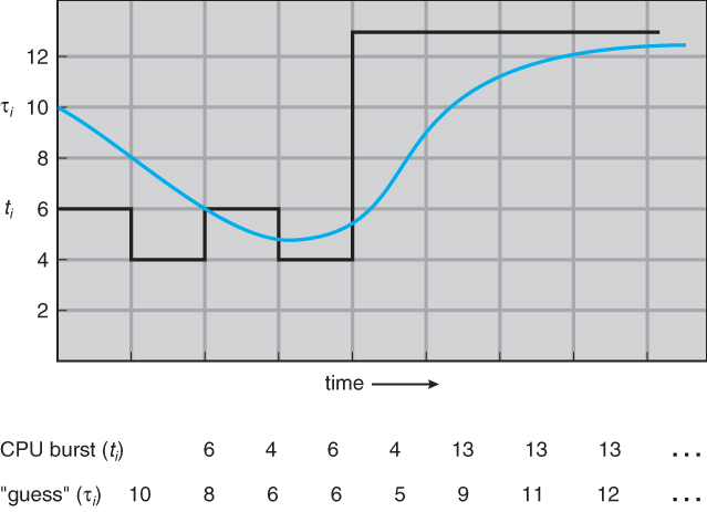
  • A more practical approach is to predict the length of the next burst, based on some historical measurement of recent burst times for this process. One simple, fast, and relatively accurate method is the exponential average, which can be defined as follows. ( The book uses tau and t for their variables, but those are hard to distinguish from one another and don't work well in HTML. )

  estimate[ i + 1 ] = alpha * burst[ i ] + ( 1.0 - alpha ) * estimate[ i ]

  • In this scheme the previous estimate contains the history of all previous times, and alpha serves as a weighting factor for the relative importance of recent data versus past history. If alpha is 1.0, then past history is ignored, and we assume the next burst will be the same length as the last burst. If alpha is 0.0, then all measured burst times are ignored, and we just assume a constant burst time. Most commonly alpha is set at 0.5, as illustrated in Figure 5.3:

Figure 6.3 - Prediction of the length of the next CPU burst.

• SJF can be either preemptive or non-preemptive. Preemption occurs when a new process arrives in the ready queue that has a predicted burst time shorter than the time remaining in the process whose burst is currently on the CPU. Preemptive SJF is sometimes referred to as shortest remaining time first scheduling.
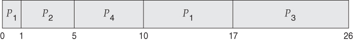
• For example, the following Gantt chart is based upon the following data:

Process Arrival Time Burst Time

• The average wait time in this case is ( ( 5 - 3 ) + ( 10 - 1 ) + ( 17 - 2 ) ) / 4 = 26 / 4 = 6.5 ms. ( As opposed to 7.75 ms for non-preemptive SJF or 8.75 for FCFS. )

6.3.3 Priority Scheduling

• Priority scheduling is a more general case of SJF, in which each job is assigned a priority and the job with the highest priority gets scheduled first. ( SJF uses the inverse of the next expected burst time as its priority - The smaller the expected burst, the higher the priority. )
• Note that in practice, priorities are implemented using integers within a fixed range, but there is no agreed-upon convention as to whether "high" priorities use large numbers or small numbers. This book uses low number for high priorities, with 0 being the highest possible priority.
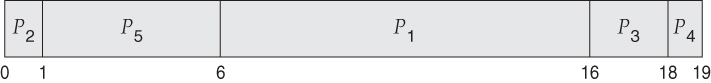
• For example, the following Gantt chart is based upon these process burst times and priorities, and yields an average waiting time of 8.2 ms:

Process Burst Time Priority

• Priorities can be assigned either internally or externally. Internal priorities are assigned by the OS using criteria such as average burst time, ratio of CPU to I/O activity, system resource use, and other factors available to the kernel. External priorities are assigned by users, based on the importance of the job, fees paid, politics, etc.
• Priority scheduling can be either preemptive or non-preemptive.
• Priority scheduling can suffer from a major problem known as indefinite blocking, or starvation, in which a low-priority task can wait forever because there are always some other jobs around that have higher priority.
  • If this problem is allowed to occur, then processes will either run eventually when the system load lightens ( at say 2:00 a.m. ), or will eventually get lost when the system is shut down or crashes. ( There are rumors of jobs that have been stuck for years. )
  • One common solution to this problem is aging, in which priorities of jobs increase the longer they wait. Under this scheme a low-priority job will eventually get its priority raised high enough that it gets run.

6.3.4 Round Robin Scheduling

• Round robin scheduling is similar to FCFS scheduling, except that CPU bursts are assigned with limits called time quantum.
• When a process is given the CPU, a timer is set for whatever value has been set for a time quantum.
  • If the process finishes its burst before the time quantum timer expires, then it is swapped out of the CPU just like the normal FCFS algorithm.
  • If the timer goes off first, then the process is swapped out of the CPU and moved to the back end of the ready queue.
• The ready queue is maintained as a circular queue, so when all processes have had a turn, then the scheduler gives the first process another turn, and so on.
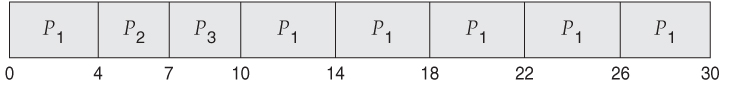
• RR scheduling can give the effect of all processors sharing the CPU equally, although the average wait time can be longer than with other scheduling algorithms. In the following example the average wait time is 5.66 ms.

Process Burst Time

• The performance of RR is sensitive to the time quantum selected. If the quantum is large enough, then RR reduces to the FCFS algorithm; If it is very small, then each process gets 1/nth of the processor time and share the CPU equally.
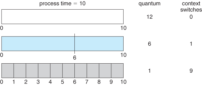
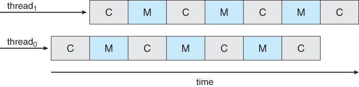
• BUT, a real system invokes overhead for every context switch, and the smaller the time quantum the more context switches there are. ( See Figure 6.4 below. ) Most modern systems use time quantum between 10 and 100 milliseconds, and context switch times on the order of 10 microseconds, so the overhead is small relative to the time quantum.

Figure 6.4 - The way in which a smaller time quantum increases context switches.

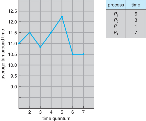
• Turn around time also varies with quantum time, in a non-apparent manner. Consider, for example the processes shown in Figure 6.5:

Figure 6.5 - The way in which turnaround time varies with the time quantum.

• In general, turnaround time is minimized if most processes finish their next cpu burst within one time quantum. For example, with three processes of 10 ms bursts each, the average turnaround time for 1 ms quantum is 29, and for 10 ms quantum it reduces to 20. However, if it is made too large, then RR just degenerates to FCFS. A rule of thumb is that 80% of CPU bursts should be smaller than the time quantum.

6.3.5 Multilevel Queue Scheduling

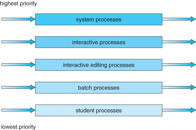
• When processes can be readily categorized, then multiple separate queues can be established, each implementing whatever scheduling algorithm is most appropriate for that type of job, and/or with different parametric adjustments.
• Scheduling must also be done between queues, that is scheduling one queue to get time relative to other queues. Two common options are strict priority ( no job in a lower priority queue runs until all higher priority queues are empty ) and round-robin ( each queue gets a time slice in turn, possibly of different sizes. )
• Note that under this algorithm jobs cannot switch from queue to queue - Once they are assigned a queue, that is their queue until they finish.

Figure 6.6 - Multilevel queue scheduling

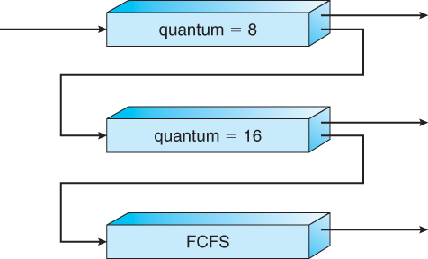
6.3.6 Multilevel Feedback-Queue Scheduling

• Multilevel feedback queue scheduling is similar to the ordinary multilevel queue scheduling described above, except jobs may be moved from one queue to another for a variety of reasons:
  • If the characteristics of a job change between CPU-intensive and I/O intensive, then it may be appropriate to switch a job from one queue to another.
  • Aging can also be incorporated, so that a job that has waited for a long time can get bumped up into a higher priority queue for a while.
• Multilevel feedback queue scheduling is the most flexible, because it can be tuned for any situation. But it is also the most complex to implement because of all the adjustable parameters. Some of the parameters which define one of these systems include:
  • The number of queues.
  • The scheduling algorithm for each queue.
  • The methods used to upgrade or demote processes from one queue to another. ( Which may be different. )
  • The method used to determine which queue a process enters initially.

Figure 6.7 - Multilevel feedback queues.

6.4 Thread Scheduling

• The process scheduler schedules only the kernel threads.
• User threads are mapped to kernel threads by the thread library - The OS ( and in particular the scheduler ) is unaware of them.

6.4.1 Contention Scope

• Contention scope refers to the scope in which threads compete for the use of physical CPUs.
• On systems implementing many-to-one and many-to-many threads, Process Contention Scope, PCS, occurs, because competition occurs between threads that are part of the same process. ( This is the management / scheduling of multiple user threads on a single kernel thread, and is managed by the thread library. )
• System Contention Scope, SCS, involves the system scheduler scheduling kernel threads to run on one or more CPUs. Systems implementing one-to-one threads ( XP, Solaris 9, Linux ), use only SCS.
• PCS scheduling is typically done with priority, where the programmer can set and/or change the priority of threads created by his or her programs. Even time slicing is not guaranteed among threads of equal priority.

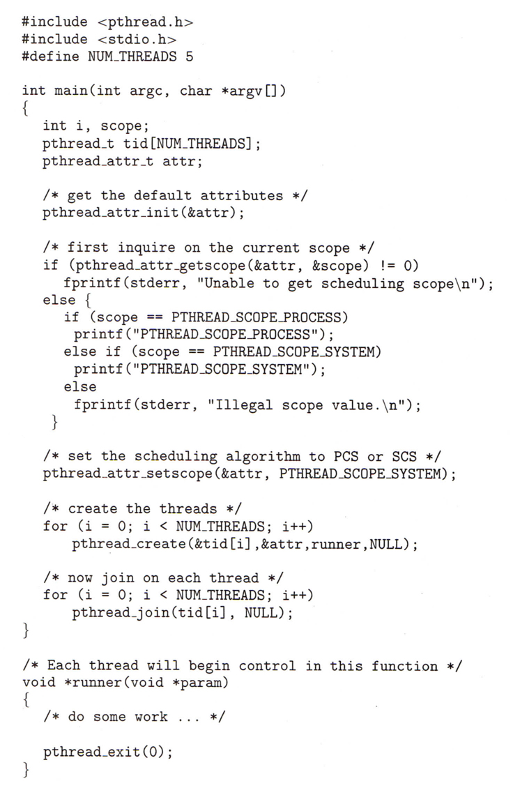
6.4.2 Pthread Scheduling

• The Pthread library provides for specifying scope contention:
  • PTHREAD_SCOPE_PROCESS schedules threads using PCS, by scheduling user threads onto available LWPs using the many-to-many model.
  • PTHREAD_SCOPE_SYSTEM schedules threads using SCS, by binding user threads to particular LWPs, effectively implementing a one-to-one model.
• getscope and setscope methods provide for determining and setting the scope contention respectively:

Figure 6.8 - Pthread scheduling API.

6.5 Multiple-Processor Scheduling

• When multiple processors are available, then the scheduling gets more complicated, because now there is more than one CPU which must be kept busy and in effective use at all times.
• Load sharing revolves around balancing the load between multiple processors.
• Multi-processor systems may be heterogeneous, ( different kinds of CPUs ), or homogenous, ( all the same kind of CPU ). Even in the latter case there may be special scheduling constraints, such as devices which are connected via a private bus to only one of the CPUs. This book will restrict its discussion to homogenous systems.

6.5.1 Approaches to Multiple-Processor Scheduling

• One approach to multi-processor scheduling is asymmetric multiprocessing, in which one processor is the master, controlling all activities and running all kernel code, while the other runs only user code. This approach is relatively simple, as there is no need to share critical system data.
• Another approach is symmetric multiprocessing, SMP, where each processor schedules its own jobs, either from a common ready queue or from separate ready queues for each processor.
• Virtually all modern OSes support SMP, including XP, Win 2000, Solaris, Linux, and Mac OSX.

6.5.2 Processor Affinity

• Processors contain cache memory, which speeds up repeated accesses to the same memory locations.
• If a process were to switch from one processor to another each time it got a time slice, the data in the cache ( for that process ) would have to be invalidated and re-loaded from main memory, thereby obviating the benefit of the cache.
• Therefore SMP systems attempt to keep processes on the same processor, via processor affinity. Soft affinity occurs when the system attempts to keep processes on the same processor but makes no guarantees. Linux and some other OSes support hard affinity, in which a process specifies that it is not to be moved between processors.
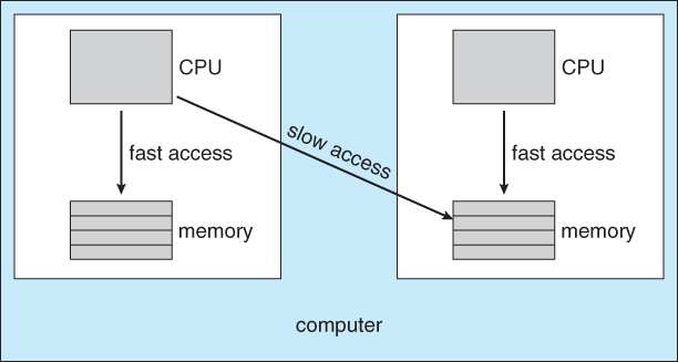
• Main memory architecture can also affect process affinity, if particular CPUs have faster access to memory on the same chip or board than to other memory loaded elsewhere. ( Non-Uniform Memory Access, NUMA. ) As shown below, if a process has an affinity for a particular CPU, then it should preferentially be assigned memory storage in "local" fast access areas.

Figure 6.9 - NUMA and CPU scheduling.

6.5.3 Load Balancing

• Obviously an important goal in a multiprocessor system is to balance the load between processors, so that one processor won't be sitting idle while another is overloaded.
• Systems using a common ready queue are naturally self-balancing, and do not need any special handling. Most systems, however, maintain separate ready queues for each processor.
• Balancing can be achieved through either push migration or pull migration:
  • Push migration involves a separate process that runs periodically, ( e.g. every 200 milliseconds ), and moves processes from heavily loaded processors onto less loaded ones.
  • Pull migration involves idle processors taking processes from the ready queues of other processors.
  • Push and pull migration are not mutually exclusive.
• Note that moving processes from processor to processor to achieve load balancing works against the principle of processor affinity, and if not carefully managed, the savings gained by balancing the system can be lost in rebuilding caches. One option is to only allow migration when imbalance surpasses a given threshold.

6.5.4 Multicore Processors

• Traditional SMP required multiple CPU chips to run multiple kernel threads concurrently.
• Recent trends are to put multiple CPUs ( cores ) onto a single chip, which appear to the system as multiple processors.
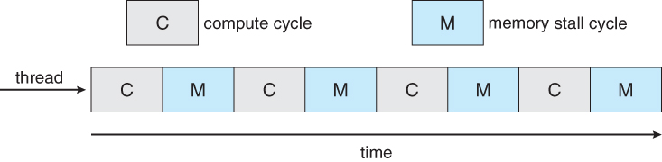
• Compute cycles can be blocked by the time needed to access memory, whenever the needed data is not already present in the cache. ( Cache misses. ) In Figure 5.10, as much as half of the CPU cycles are lost to memory stall.

Figure 6.10 - Memory stall.

• By assigning multiple kernel threads to a single processor, memory stall can be avoided ( or reduced ) by running one thread on the processor while the other thread waits for memory.

Figure 6.11 - Multithreaded multicore system.

• A dual-threaded dual-core system has four logical processors available to the operating system. The UltraSPARC T1 CPU has 8 cores per chip and 4 hardware threads per core, for a total of 32 logical processors per chip.
• There are two ways to multi-thread a processor:
  1. Coarse-grained multithreading switches between threads only when one thread blocks, say on a memory read. Context switching is similar to process switching, with considerable overhead.
  2. Fine-grained multithreading occurs on smaller regular intervals, say on the boundary of instruction cycles. However the architecture is designed to support thread switching, so the overhead is relatively minor.
• Note that for a multi-threaded multi-core system, there are two levels of scheduling, at the kernel level:
  • The OS schedules which kernel thread(s) to assign to which logical processors, and when to make context switches using algorithms as described above.
  • On a lower level, the hardware schedules logical processors on each physical core using some other algorithm.
    • The UltraSPARC T1 uses a simple round-robin method to schedule the 4 logical processors ( kernel threads ) on each physical core.
    • The Intel Itanium is a dual-core chip which uses a 7-level priority scheme ( urgency ) to determine which thread to schedule when one of 5 different events occurs.

/* Old 5.5.5 Virtualization and Scheduling ( Optional, Omitted from 9th edition )

• Virtualization adds another layer of complexity and scheduling.
• Typically there is one host operating system operating on "real" processor(s) and a number of guest operating systems operating on virtual processors.
• The Host OS creates some number of virtual processors and presents them to the guest OSes as if they were real processors.
• The guest OSes don't realize their processors are virtual, and make scheduling decisions on the assumption of real processors.
• As a result, interactive and especially real-time performance can be severely compromised on guest systems. The time-of-day clock will also frequently be off.

6.6 Real-Time CPU Scheduling

Real-time systems are those in which the time at which tasks complete is crucial to their performance

• Soft real-time systems have degraded performance if their timing needs cannot be met. Example: streaming video.
• Hard real-time systems have total failure if their timing needs cannot be met. Examples: Assembly line robotics, automobile air-bag deployment.

6.6.1 Minimizing Latency

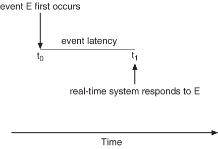
• Event Latency is the time between the occurrence of a triggering event and the ( completion of ) the system's response to the event:

Figure 6.12 - Event latency.

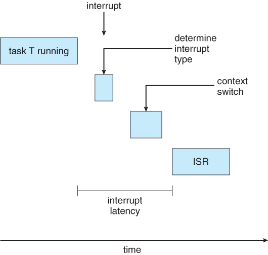
• In addition to the time it takes to actually process the event, there are two additional steps that must occur before the event handler ( Interrupt Service Routine, ISR ), can even start:
  • Interrupt processing determines which interrupt(s) have occurred, and which interrupt handler routine to run. In the event of simultaneous interrupts, a priority scheme is needed to determine which ISR has the highest priority and gets to go next.
  • Context switching involves removing a running process from the CPU, saving its state, and loading up the ISR so that it can run.

Figure 6.13 - Interrupt latency.

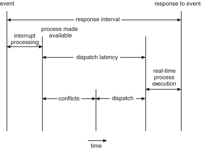
• • The total dispatch latency ( context switching ) consists of two parts:
    • Removing the currently running process from the CPU, and freeing up any resources that are needed by the ISR. This step can be speeded up a lot by the use of pre-emptive kernels.
    • Loading the ISR up onto the CPU, ( dispatching )

Figure 6.14 - Dispatch latency.

6.6.2 Priority-Based Scheduling

• Real-time systems require pre-emptive priority-based scheduling systems.
• Soft real-time systems do the best they can, but make no guarantees. They are generally discussed elsewhere.
• Hard real-time systems, described here, must be able to provide firm guarantees that a tasks scheduling needs can be met.
  • One technique is to use a admission-control algorithm, in which each task must specify its needs at the time it attempts to launch, and the system will only launch the task if it can guarantee that its needs can be met.
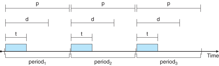
• Hard real-time systems are often characterized by tasks that must run at regular periodic intervals, each having a period p, a constant time required to execute, ( CPU burst ), t, and a deadline after the beginning of each period by which the task must be completed, d.
• In all cases, t <= d <= p

Figure 6.15 - Periodic task.

6.6.3 Rate-Monotonic Scheduling

• The rate-monotonic scheduling algorithm uses pre-emptive scheduling with static priorities.
• Priorities are assigned inversely to the period of each task, giving higher ( better ) priority to tasks with shorter periods.
• Let's consider an example, first showing what can happen if the task with the longer period is given higher priority:
  • Suppose that process P1 has a period of 50, an execution time of 20, and a deadline that matches its period ( 50 ).
  • Similarly suppose that process P2 has period 100, execution time of 35, and deadline of 100.
  • The total CPU utilization time is 20 / 50 = 0.4 for P1, and 25 / 100 = 0.35 for P2, or 0.75 ( 75% ) overall.
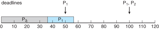
  • However if P2 is allowed to go first, then P1 cannot complete before its deadline:

Figure 6.16 - Scheduling of tasks when P2 has a higher priority than P1.

• • Now on the other hand, if P1 is given higher priority, it gets to go first, and P2 starts after P1 completes its burst.
  • At time 50 when the next period for P1 starts, P2 has only completed 30 of its 35 needed time units, but it gets pre-empted by P1.
  • At time 70, P1 completes its task for its second period, and the P2 is allowed to complete its last 5 time units.
  • Overall both processes complete at time 75, and the cpu is then idle for 25 time units, before the process repeats.

Figure 6.17 - Rate-monotonic scheduling.

• • Rate-monotonic scheduling is considered optimal among algorithms that use static priorities, because any set of processes that cannot be scheduled with this algorithm cannot be scheduled with any other static-priority scheduling algorithm either.
  • There are, however, some sets of processes that cannot be scheduled with static priorities.
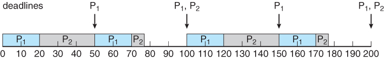
    • For example, supposing that P1 =50, T1 = 25, P2 = 80, T2 = 35, and the deadlines match the periods.
    • Overall CPU usage is 25/50 = 0.5 for P1, 35 / 80 =0.44 for P2, or 0.94 ( 94% ) overall, indicating it should be possible to schedule the processes.
    • With rate-monotonic scheduling, P1 goes first, and completes its first burst at time 25.
    • P2 goes next, and completes 25 out of its 35 time units before it gets pre-empted by P1 at time 50.
    • P1 completes its second burst at 75, and then P2 completes its last 10 time units at time 85, missing its deadline of 80 by 5 time units. :-(

Figure 6.18 - Missing deadlines with rate-monotonic scheduling.

• • The worst-case CPU utilization for scheduling N processes under this algorithm is N * ( 2^(1/N) - 1 ), which is 100% for a single process, but drops to 75% for two processes and to 69% as N approaches infinity. Note that in our example above 94% is higher than 75%.

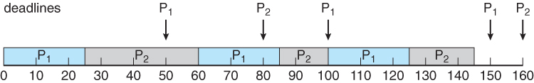
6.6.4 Earliest-Deadline-First Scheduling

• Earliest Deadline First ( EDF ) scheduling varies priorities dynamically, giving the highest priority to the process with the earliest deadline.
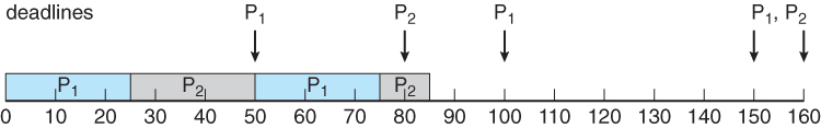
• Figure 6.19 shows our previous example repeated under EDF scheduling:
  • At time 0 P1 has the earliest deadline, highest priority, and goes first., followed by P2 at time 25 when P1 completes its first burst.
  • At time 50 process P1 begins its second period, but since P2 has a deadline of 80 and the deadline for P1 is not until 100, P2 is allowed to stay on the CPU and complete its burst, which it does at time 60.
  • P1 then starts its second burst, which it completes at time 85. P2 started its second period at time 80, but since P1 had an earlier deadline, P2 did not pre-empt P1.
  • P2 starts its second burst at time 85, and continues until time 100, at which time P1 starts its third period.
  • At this point P1 has a deadline of 150 and P2 has a deadline of 160, so P1 preempts P2.
  • P1 completes its third burst at time 125, at which time P2 starts, completing its third burst at time 145.
  • The CPU sits idle for 5 time units, until P1 starts its next period at 150 and P2 at 160.
  • Question: Which process will get to run at time 160, and why?
    • Answer: Process P2, because P1 now has a deadline of 200 and P2's new deadline is 240.

Figure 6.19 - Earliest-deadline-first scheduling.

6.6.5 Proportional Share Scheduling

• Proportional share scheduling works by dividing the total amount of time available up into an equal number of shares, and then each process must request a certain share of the total when it tries to start.
• Say for example that the total shares, T, = 100, and then a particular process asks for N = 30 shares when it launches. It will then be guaranteed 30 / 100 or 30% of the available time.
• Proportional share scheduling works with an admission-control policy, not starting any task if it cannot guarantee the shares that the task says that it needs.

6.6.6 POSIX Real-Time Scheduling

• POSIX defines two scheduling classes for real time threads, SCHED_FIFO and SCHED_RR, depending on how threads of equal priority share time.
• SCHED_FIFO schedules tasks in a first-in-first-out order, with no time slicing among threads of equal priority.
• SCHED_RR performs round-robin time slicing among threads of equal priority.
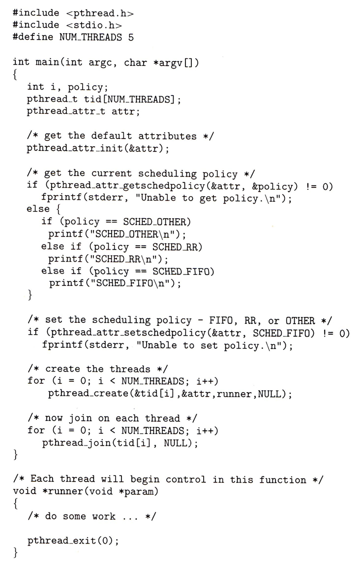
• POSIX provides methods for getting and setting the thread scheduling policy, as shown below:

Figure 6.20 - POSIX real-time scheduling API.

6.7 Operating System Examples ( Optional )

6.7.1 Example: Linux Scheduling ( was 5.6.3 )

• Prior to version 2.5, Linux used a traditional UNIX scheduling algorithm.
• Version 2.6 used an algorithm known as O(1), that ran in constant time regardless of the number of tasks, and provided better support for SMP systems. However it yielded poor interactive performance.
• Starting in 2.6.23, the Completely Fair Scheduler, CFS, became the standard Linux scheduling system. See sidebar below

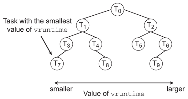
CFS ( Completely Fair Scheduler ) Performance

The Linux CFS scheduler provides an efficient algorithm for selecting which
task to run next. Each runnable task is placed in a red-black tree—a balanced
binary search tree whose key is based on the value of vruntime. This tree is
shown below:

When a task becomes runnable, it is added to the tree.  If a task on the
tree is not runnable ( for example, if it is blocked while waiting for I/O ), it is
removed.  Generally speaking, tasks that have been given less processing time
( smaller values of vruntime ) are toward the left side of the tree, and tasks
that have been given more processing time are on the right side. According
to the properties of a binary search tree, the leftmost node has the smallest
key value, which for the sake of the CFS scheduler means that it is the task
with the highest priority . Because the red-black tree is balanced, navigating
it to discover the leftmost node will require O(lgN) operations (where N
is the number of nodes in the tree). However, for efficiency reasons, the
Linux scheduler caches this value in the variable rb_leftmost, and thus
determining which task to run next requires only retrieving the cached value.

New sidebar in ninth edition

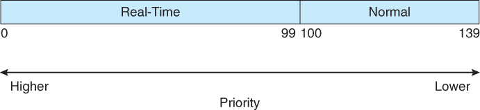
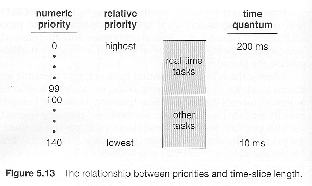
• The Linux scheduler is a preemptive priority-based algorithm with two priority ranges - Real time from 0 to 99 and a nice range from 100 to 140.
• Unlike Solaris or XP, Linux assigns longer time quantums to higher priority tasks.

Figure 6.21 - Scheduling priorities on a Linux system.

Replaced by Figure 6.21 in the ninth edition. Was Figure 5.15 in eighth edition

/* The Following material was omitted from the ninth edition:

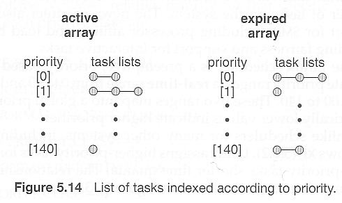
• • A runnable task is considered eligible for execution as long as it has not consumed all the time available in it's time slice. Those tasks are stored in an active array, indexed according to priority.
  • When a process consumes its time slice, it is moved to an expired array. The tasks priority may be re-assigned as part of the transferal.
  • When the active array becomes empty, the two arrays are swapped.
  • These arrays are stored in runqueue structures. On multiprocessor machines, each processor has its own scheduler with its own runqueue.

Omitted from ninth edition. Figure 5.16 in eighth edition.

6.7.2 Example: Windows XP Scheduling ( was 5.6.2 )

• Windows XP uses a priority-based preemptive scheduling algorithm.
• The dispatcher uses a 32-level priority scheme to determine the order of thread execution, divided into two classes - variable class from 1 to 15 and real-time class from 16 to 31, ( plus a thread at priority 0 managing memory. )
• There is also a special idle thread that is scheduled when no other threads are ready.
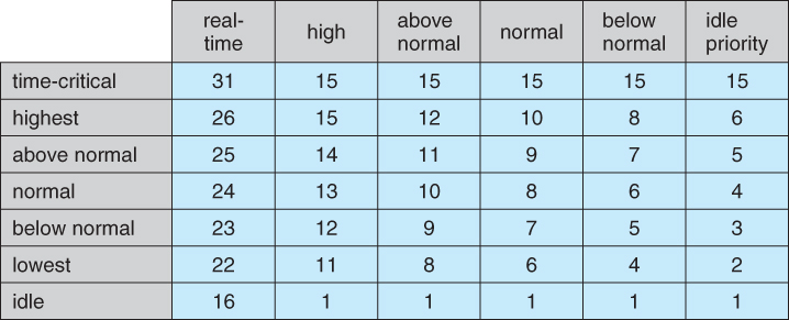
• Win XP identifies 7 priority classes ( rows on the table below ), and 6 relative priorities within each class ( columns. )
• Processes are also each given a base priority within their priority class. When variable class processes consume their entire time quanta, then their priority gets lowered, but not below their base priority.
• Processes in the foreground ( active window ) have their scheduling quanta multiplied by 3, to give better response to interactive processes in the foreground.

Figure 6.22 - Windows thread priorities.

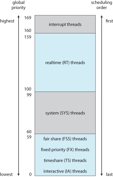
6.7.1 Example: Solaris Scheduling

• Priority-based kernel thread scheduling.
• Four classes ( real-time, system, interactive, and time-sharing ), and multiple queues / algorithms within each class.
• Default is time-sharing.
  • Process priorities and time slices are adjusted dynamically in a multilevel-feedback priority queue system.
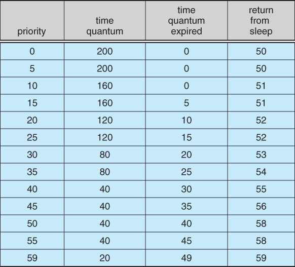
  • Time slices are inversely proportional to priority - Higher priority jobs get smaller time slices.
  • Interactive jobs have higher priority than CPU-Bound ones.
  • See the table below for some of the 60 priority levels and how they shift. "Time quantum expired" and "return from sleep" indicate the new priority when those events occur. ( Larger numbers are a higher, i.e. better priority. )

Figure 6.23 - Solaris dispatch table for time-sharing and interactive threads.

• Solaris 9 introduced two new scheduling classes: Fixed priority and fair share.
  • Fixed priority is similar to time sharing, but not adjusted dynamically.
  • Fair share uses shares of CPU time rather than priorities to schedule jobs. A certain share of the available CPU time is allocated to a project, which is a set of processes.
• System class is reserved for kernel use. ( User programs running in kernel mode are NOT considered in the system scheduling class. )

Figure 6.24 - Solaris scheduling.

6.8 Algorithm Evaluation

• The first step in determining which algorithm ( and what parameter settings within that algorithm ) is optimal for a particular operating environment is to determine what criteria are to be used, what goals are to be targeted, and what constraints if any must be applied. For example, one might want to "maximize CPU utilization, subject to a maximum response time of 1 second".
• Once criteria have been established, then different algorithms can be analyzed and a "best choice" determined. The following sections outline some different methods for determining the "best choice".

6.8.1 Deterministic Modeling

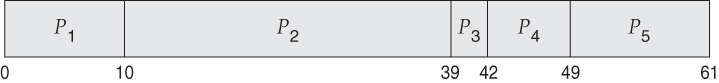
• If a specific workload is known, then the exact values for major criteria can be fairly easily calculated, and the "best" determined. For example, consider the following workload ( with all processes arriving at time 0 ), and the resulting schedules determined by three different algorithms:

Process Burst Time

FCFS:

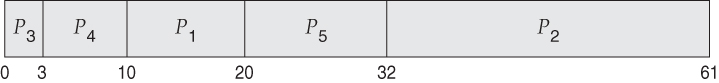
Non-preemptive SJF:

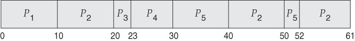
Round Robin:

• The average waiting times for FCFS, SJF, and RR are 28ms, 13ms, and 23ms respectively.
• Deterministic modeling is fast and easy, but it requires specific known input, and the results only apply for that particular set of input. However by examining multiple similar cases, certain trends can be observed. ( Like the fact that for processes arriving at the same time, SJF will always yield the shortest average wait time. )

6.8.2 Queuing Models

• Specific process data is often not available, particularly for future times. However a study of historical performance can often produce statistical descriptions of certain important parameters, such as the rate at which new processes arrive, the ratio of CPU bursts to I/O times, the distribution of CPU burst times and I/O burst times, etc.
• Armed with those probability distributions and some mathematical formulas, it is possible to calculate certain performance characteristics of individual waiting queues. For example, Little's Formula says that for an average queue length of N, with an average waiting time in the queue of W, and an average arrival of new jobs in the queue of Lambda, then these three terms can be related by:

N = Lambda * W

• Queuing models treat the computer as a network of interconnected queues, each of which is described by its probability distribution statistics and formulas such as Little's formula. Unfortunately real systems and modern scheduling algorithms are so complex as to make the mathematics intractable in many cases with real systems.

6.8.3 Simulations

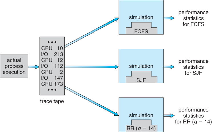
• Another approach is to run computer simulations of the different proposed algorithms ( and adjustment parameters ) under different load conditions, and to analyze the results to determine the "best" choice of operation for a particular load pattern.
• Operating conditions for simulations are often randomly generated using distribution functions similar to those described above.
• A better alternative when possible is to generate trace tapes, by monitoring and logging the performance of a real system under typical expected work loads. These are better because they provide a more accurate picture of system loads, and also because they allow multiple simulations to be run with the identical process load, and not just statistically equivalent loads. A compromise is to randomly determine system loads and then save the results into a file, so that all simulations can be run against identical randomly determined system loads.
• Although trace tapes provide more accurate input information, they can be difficult and expensive to collect and store, and their use increases the complexity of the simulations significantly. There is also some question as to whether the future performance of the new system will really match the past performance of the old system. ( If the system runs faster, users may take fewer coffee breaks, and submit more processes per hour than under the old system. Conversely if the turnaround time for jobs is longer, intelligent users may think more carefully about the jobs they submit rather than randomly submitting jobs and hoping that one of them works out. )

Figure 6.25 - Evaluation of CPU schedulers by simulation.

6.8.4 Implementation

• The only real way to determine how a proposed scheduling algorithm is going to operate is to implement it on a real system.
• For experimental algorithms and those under development, this can cause difficulties and resistance among users who don't care about developing OSes and are only trying to get their daily work done.
• Even in this case, the measured results may not be definitive, for at least two major reasons: (1) System work loads are not static, but change over time as new programs are installed, new users are added to the system, new hardware becomes available, new work projects get started, and even societal changes. ( For example the explosion of the Internet has drastically changed the amount of network traffic that a system sees and the importance of handling it with rapid response times. ) (2) As mentioned above, changing the scheduling system may have an impact on the work load and the ways in which users use the system. ( The book gives an example of a programmer who modified his code to write an arbitrary character to the screen at regular intervals, just so his job would be classified as interactive and placed into a higher priority queue. )
• Most modern systems provide some capability for the system administrator to adjust scheduling parameters, either on the fly or as the result of a reboot or a kernel rebuild.

6.9 Summary

Material Omitted from the Eighth Edition:

Was 5.4.4 Symmetric Multithreading ( Omitted from 8th edition )

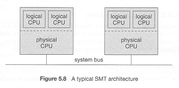
• An alternative strategy to SMP is SMT, Symmetric Multi-Threading, in which multiple virtual ( logical ) CPUs are used instead of ( or in combination with ) multiple physical CPUs.
• SMT must be supported in hardware, as each logical CPU has its own registers and handles its own interrupts. ( Intel refers to SMT as hyperthreading technology. )
• To some extent the OS does not need to know if the processors it is managing are real or virtual. On the other hand, some scheduling decisions can be optimized if the scheduler knows the mapping of virtual processors to real CPUs. ( Consider the scheduling of two CPU-intensive processes on the architecture shown below. )

omitted