Mar 14, 2016

Leapfrog Probing

A hash table is a data structure that stores a set of items, each of which maps a specific key to a specific value. There are many ways to implement a hash table, but they all have one thing in common: buckets. Every hash table maintains an array of buckets somewhere, and each item belongs to exactly one bucket.

To determine the bucket for a given item, you typically hash the item’s key, then compute its modulus – that is, the remainder when divided by the number of buckets. For a hash table with 16 buckets, the modulus is given by the final hexadecimal digit of the hash.

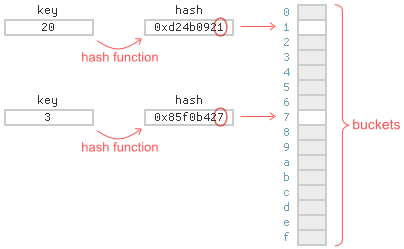
Inevitably, several items will end up belonging to same bucket. For simplicity, let’s suppose the hash function is invertible, so that we only need to store hashed keys. A well-known strategy is to store the bucket contents in a linked list:

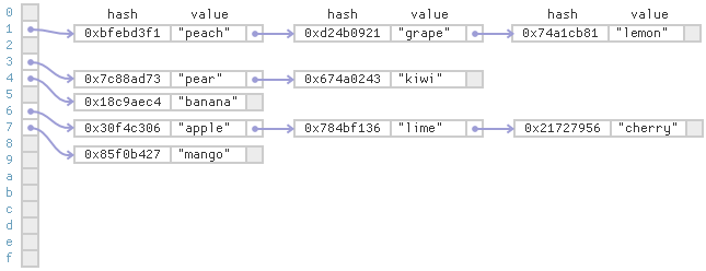
This strategy is known as separate chaining. Separate chaining tends to be relatively slow on modern CPUs, since it requires a lot of pointer lookups.

I’m more fond of open addressing, which stores all the items in the array itself:

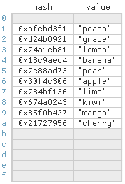
In open addressing, each cell in the array still represents a single bucket, but can actually store an item belonging to any bucket. Open addressing is more cache-friendly than separate chaining. If an item is not found in its ideal cell, it’s often nearby. The drawback is that as the array becomes full, you may need to search a lot of cells before finding a particular item, depending on the probing strategy.

For example, consider linear probing, the simplest probing strategy. Suppose we want to insert the item (13, “orange”) into the above table, and the hash of 13 is 0x95bb7d92. Ideally, we’d store this item at index 2, the last hexadecimal digit of the hash, but that cell is already taken. Under linear probing, we find the next free cell by searching linearly, starting at the item’s ideal index, and store the item there instead:

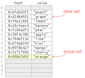
As you can see, the item (13, “orange”) ended up quite far from its ideal cell. Not great for lookups. Every time someone calls get with this key, they’ll have to search cells 2 through 11 before finding it. As the array becomes full, long searches become more and more common. Nonetheless, linear probing tends to be quite fast as long as you don’t let the array get too full. I’ve shown benchmarks in previous posts.

There are alternatives to linear probing, such as quadratic probing, double hashing, cuckoo hashing and hopscotch hashing. While developing Junction, I came up with yet another strategy. I call it leapfrog probing. Leapfrog probing reduces the average search length compared to linear probing, while also lending itself nicely to concurrency. It was inspired by hopscotch hashing, but uses explicit delta values instead of bitfields to identify cells belonging to a given bucket.

Finding Existing Items

In leapfrog probing, we store two additional delta values for each cell. These delta values define an explicit probe chain for each bucket.

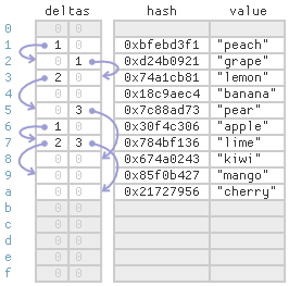
To find a given key, proceed as follows:

1. First, hash the key and compute its modulus to get the bucket index. That’s the item’s ideal cell. Check there first.
2. If the item isn’t found in that cell, use that cell’s first delta value to determine the next cell to check. Just add the delta value to the current array index, making sure to wrap at the end of the array.
3. If the item isn’t found in that cell, use the second delta value for all subsequent cells. Stop when the delta is zero.

For the strategy to work, there really needs to be two delta values per cell. The first delta value directs us to the desired bucket’s probe chain (if not already in it), and the second delta value keeps us in the same probe chain.

For example, suppose we look for the key 40 in the above table, and 40 hashes to 0x674a0243. The modulus (last digit) is 3, so we check index 3 first, but index 3 contains an item belonging to a different bucket. The first delta value at index 3 is 2, so we add that to the current index and check index 5. The item isn’t there either, but at least index 5 contains an item belonging to the desired bucket, since its hash also ends with 3. The second delta value at index 5 is 3, so we add that to the current index and check index 8. At index 8, the hashed key 0x674a0243 is found.

A single byte is sufficient to store each delta value. If the hash table’s keys and values are 4 bytes each, and we pack the delta values together, it only takes 25% additional memory to add them. If the keys and values are 8 bytes, the additional memory is just 12.5%. Best of all, we can let the hash table become much more full before having to resize.

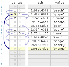
Inserting New Items

Inserting an item into a leapfrog table consists of two phases: following the probe chain to see if an item with the same key already exists, then, if not, performing a linear search for a free cell. The linear search begins at the end of the probe chain. Once a free cell is found and reserved, it gets linked to the end of the chain.

For example, suppose we insert the same item (13, “orange”) we inserted earlier, with hash 0x95bb7d92. This item’s bucket index is 2, but index 2 already contains a different key. The first delta value at index 2 is zero, which marks the end of the probe chain. We proceed to the second phase: performing a linear search starting at index 2 to locate the next free cell. As before, the item ends up quite far from its ideal cell, but this time, we set index 2’s first delta value to 9, linking the item to its probe chain. Now, subsequent lookups will find the item more quickly.

Of course, any time we search for a free cell, the cell must fall within reach of its designated probe chain. In other words, the resulting delta value must fit into a single byte. If the delta value doesn’t fit, then the table is overpopulated, and it’s time to migrate its entire contents to a new table.

In you’re interested, I added a single-threaded leapfrog map to Junction. The single-threaded version is easier to follow than the concurrent one, if you’d just like to study how leapfrog probing works.

Concurrent Operations

Junction also contains a concurrent leapfrog map. It’s the most interesting map to talk about, so I’ll simply refer to it as Leapfrog from this point on.

Leapfrog is quite similar to Junction’s concurrent Linear map, which I described in the previous post. In Leapfrog, (hashed) keys are assigned to cells in the same way that Linear would assign them, and once a cell is reserved for a key, that cell’s key never changes as long as the table is in use. The delta values are nothing but shortcuts between keys; they’re entirely determined by key placement.

In Leapfrog, reserving a cell and linking that cell to its probe chain are two discrete steps. First, the cell is reserved via compare-and-swap (CAS). If that succeeds, the cell is then linked to the end of its probe chain using a relaxed atomic store:

    ...
    while (linearProbesRemaining-- > 0) {
        idx++;
        group = table->getCellGroups() + ((idx & sizeMask) >> 2);
        cell = group->cells + (idx & 3);
        probeHash = cell->hash.load(turf::Relaxed);
        if (probeHash == KeyTraits::NullHash) {
            // It's an empty cell. Try to reserve it.
            if (cell->hash.compareExchangeStrong(probeHash, hash, turf::Relaxed)) {
                // Success. We've reserved the cell. Link it to previous cell in same bucket.
                u8 desiredDelta = idx - prevLinkIdx;
                prevLink->store(desiredDelta, turf::Relaxed);
                return InsertResult_InsertedNew;
            }
        }
        ...

Each step is atomic on its own, but together, they’re not atomic. That means that if another thread performs a concurrent operation, one of the steps could be visible but not the other. Leapfrog operations must account for all possibilities.

For example, suppose Thread 1 inserts (18, “fig”) into the table shown earlier, and 18 hashes to 0xd6045317. This item belongs in bucket 7, so it will ultimately get linked to the existing “mango” item at index 9, which was the last item belonging to the same bucket.

Now, suppose Thread 2 performs a concurrent get with the same key. It’s totally possible that, during the get, Thread 1’s link from index 9 will be visible, but not the new item itself:

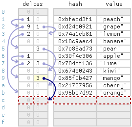
In this case, Leapfrog simply lets the concurrent get return NullValue, meaning the key wasn’t found. This is perfectly OK, since the insert and the get are concurrent. In other words, they’re racing. We aren’t obligated to ensure the newly inserted item is visible in this case. For a well-behaved concurrent map, we only need to ensure visibility when there’s a happens-before relationship between two operations, not when they’re racing.

Concurrent inserts require a bit more care. For example, suppose Thread 3 performs a concurrent insert of (62, “plum”) while Thread 1 is inserting (18, “fig”), and 62 hashes to 0x95ed72b7. In this case, both items belong to the same bucket. Again, it’s totally possible that from Thread 3’s point of view, the link from index 9 is visible, but not Thread 1’s new item, as illustrated above.

We can’t allow Thread 3 to continue any further at this point. Thread 3 absolutely needs to know whether Thread 1’s new item uses the same hashed key – otherwise, it could end up inserting a second copy of the same hashed key into the table. In Leapfrog, when this case is detected, Thread 3 simply spin-reads until the new item becomes visible before proceeding.

The opposite order is possible, too. During Thread 2’s concurrent get, Thread 1’s link from index 9 might not be visible even though the item itself is already visible:

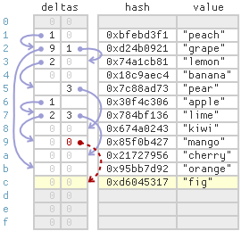
In this case, the concurrent get will simply consider index 9 to be the end of the probe chain and return NullValue, meaning the key wasn’t found. This, too, is perfectly OK. Again, Thread 1 and Thread 2 are in a race, and we aren’t obligated to ensure the insert is visible to the get.

Once again, concurrent inserts require a bit more care. If Thread 3 performs a concurrent insert into the same bucket as Thread 1, and Thread 1’s link from index 9 is not yet visible, Thread 3 will consider index 9 to be the end of the probe chain, then switch to a linear search for a free cell. During the linear search, Thread 3 might encounter Thread 1’s item (18, “fig”), as illustrated above. The item is unexpected during the linear search, because normally, items in the same bucket should be linked to the same probe chain.

In Leapfrog, when this case is detected, Thread 3 takes matters into its own hands: It sets the link from index 9 on behalf of Thread 1! This is obviously redundant, since both threads will end up writing the same delta value at roughly the same time, but it’s important. If Thread 3 doesn’t set the link from index 9, it could then call get with key 62, and if the link is still not visible, the item (62, “plum”) it just inserted will not be found.

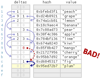
That’s bad behavior, because sequential operations performed by a single thread should always be visible to each other. I actually encountered this bug during testing.

In the benchmarks I posted earlier, Leapfrog was the fastest concurrent map out of all the concurrent maps I tested, at least up to a modest number of CPU cores. I suspect that part of its speed comes from leapfrog probing, and part comes from having very low write contention on shared variables. In particular, Leapfrog doesn’t keep track of the map’s population anywhere, since the decision to resize is based on failed inserts, not on the map’s population.