Impossible but true: a new approach to linear systems

Prasad Raghavendra is an expert in many aspects of complexity theory, especially the foundations of approximation theory. He recently was a colleague at Georgia Tech, but now has moved on to Berkeley. He will be greatly missed at Tech.

Today I want to talk about a brilliant new result that Prasad has on linear equations.

I was recently at the advisory meeting for the Berkeley Simons Theory Institute. During the meeting we had two presentations on new areas, besides talks on planned special projects. One was given by Prasad on theory, but almost in passing he mentioned that he had a way to solve linear systems. I liked the whole talk, but his almost causal comment surprised me. It seemed to me to be an entire new approach to solving linear systems. My initial thought was it must be something well known, but I did not know it.

As soon as he finished his talk we had a break, and I ran up to thank him for a wonderful talk. I quickly asked was his result on linear systems new? Or was it something I had missed? He answered to several of us, who now were waiting to hear his answer, that it was something that he had just proved. I was relieved: I am not completely out of it.

I asked if we could write about this result and he agreed. Even better, he wrote up a draft paper with just the algorithm and its analysis, which are part of larger results and projects that were the body of his talk.

Solving Linear Systems

The solving of linear systems of equations is ancient, dating back to 600 BCE. It is of extreme importance, and still an active area of research. For arbitrary systems Gaussian Elimination is still quite powerful. A historical note, apparently Carl Gauss only used the method named after him on six-variable problems. In those days there was no notion of, I can solve the general case in time cubic in . There was no “n”: of course there was the letter “n,” but not the notion of solving a problem of size determined by .

Of course now we have faster methods than this for general systems, methods that descend from the famous breakthrough of Volker Strassen. For special systems there are almost-linear-time methods, but these all require that the system have special structure, and work over the reals.

The Idea, and a Problem

Prasad’s work is for solving linear systems over finite fields, specifically with prime. For example, consider these equations over the field of two elements:

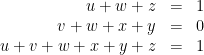
Such systems are of great importance in theory, and it shocked me that he found an entirely new approach to solving them. Note that Gaussian elimination happens to work well in this example: the second and third equations yield , and this gives . However, in general this requires sifting through each equation multiple times, and defines all the solutions. Can we do better by considering each equation only once, and by needing only some solution?

So what does he do?

He starts with a random set of vectors . Then he checks which ones satisfy the first equation. If the vectors are random, then about half of them will satisfy the equation. He throws away all the vectors that do not satisfy the equation. Call the remaining set . This is not a typo—we have a reason for using not —you will see soon.

The obvious idea is to iterate with on the second equation: About half the vectors in will satisfy it; let be those that do. Vectors in still satisfy the first equation, so the winnowing-down process that continues by taking the vectors in that satisfy the third equation finds solutions to all considered equations. The problem is that with high probability it winnows down to zero before all equations are satisfied—unless you start with having order-of vectors, which is too many.

How to solve this problem? The surprising answer is that one doesn’t need to start with a large initial to maintain a high probability of catching a solution to all the equations. It suffices to maintain a suitable large-enough set of solutions to the first equations. But how does he do this?

The Amplifier, and a Trick

The key is to use an amplifier of the kind we discussed here. After he takes the subset of , he rebuilds a set of the same size as by taking combinations of vectors in that are “random enough.” Then he proceeds on to the next equation. In this way he gets a series of sets of vectors,

so that satisfies the first equations, the sets are large, and they are almost random. The last set is nonempty with high probability, and so has a solution to the linear system.

To make this work he needs one trick, and this is why the result is limited to finite fields. To see it, first note that if all the equations are set equal to zero, then any linear combination of solutions will be a solution. If the constants are non-zero, however, this fails. For instance in the above equations, the all-1 vector satisfies the first two, as does the vector with and flipped to . The sum of these vectors, which has and the other variables , fails to satisfy the first equation.

The trick is that if you sum three solutions to the first two equations, then you always get a solution to both. Generally over with characteristic , the trick is to form random sums of vectors. The point is these vectors all satisfy some equation

then the sum of vectors will give on the right-hand side. But in characteristic , . Hence the original equation remains satisfied.

The algorithm to form from while still satisfying the th equation—and all equations before it—is just to form random sums of vectors in until has been amplified to the needed size.

So that is how he does it. Pretty cool?

He calls the amplification step a “recombination” step. Essentially he picks random vectors and adds them together. The evolutionary analogy is that this process performs enough “mixing” to preserve the needed amount of entropy.

The Algorithm

Here is the actual algorithm from his paper draft.

As always see his paper for the details and full proof that the method works. This is the hard part. I take that back, both the creation of the algorithm and its proof of correctness are equally tricky. Indeed the fact that there is a new algorithm is perhaps most surprising of all.

Open Problems

This approach of guess, delete, recombine reminds me of what are sometimes called genetic algorithms. Are there applications of Prasad algorithm? Or of his general method to other problems?