

Focusing on Focal Mechanisms with Python
source link: https://hackernoon.com/focusing-on-focal-mechanisms-with-python
Go to the source link to view the article. You can view the picture content, updated content and better typesetting reading experience. If the link is broken, please click the button below to view the snapshot at that time.
Focusing on Focal Mechanisms with Python
A comprehensive tutorial for plotting focal mechanism "beach-balls" using the PyGMT package for Python. The walk-through covers downloading focal mechanism data from the SCEDC, conditioning the data, creating a postscript legend, and plotting everything on a map.
Highlights include: - Offsetting "beach-balls" from their point of origin - Scaling "beach-balls" by magnitude - Coloring "beach-balls" by depth - Plotting label text above each "beach-ball" - Controlling the size of the label text - Automatically downloading an SRTM DEM - Creating a postscript legend file
@boaFirst Try
Learning new things and sharing them
To better understand the faulting motions that create earthquakes, it can be useful to graphically display focal mechanisms. A focal mechanism is the orientation and type of slip of a fault, and it is represented as a “beach-ball” symbol.
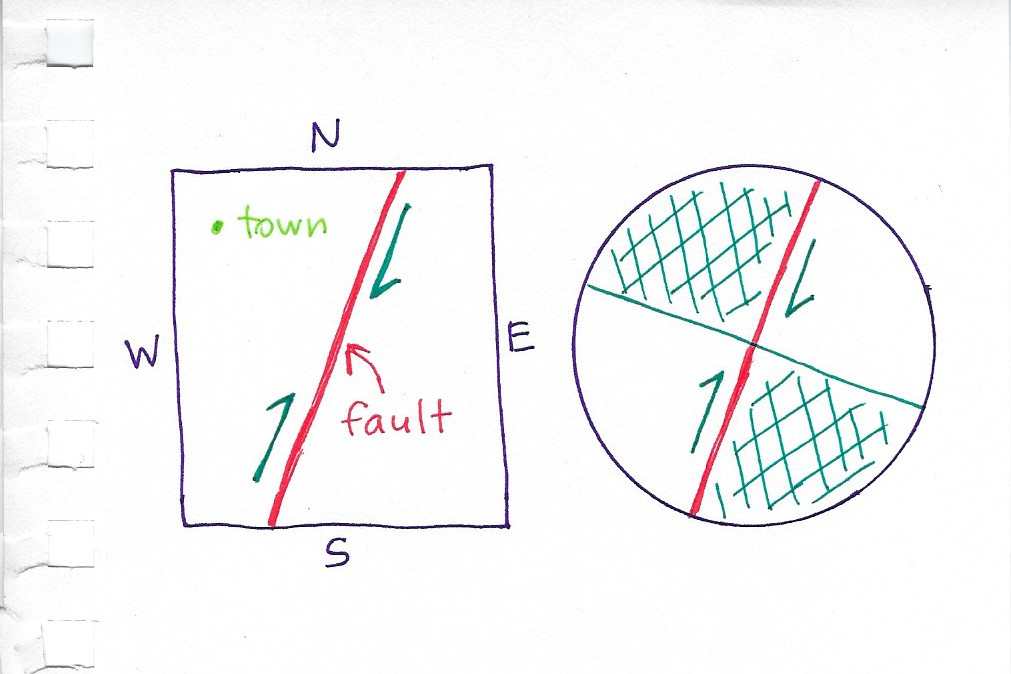
Image is sourced from the United States Geological Survey earthquake hazards webpage on focal mechanisms
Within a “beach-ball,” the dark quarters represent compressional forces and the white quarters represent tensional forces. A “beach-ball” has two possible orientations of fault movement, each along with one of the planes dividing the “beach-ball” into fourths, and determining the correct orientation requires additional information. When “beach-balls” present four equally sized quadrants in a “top-down” view like the one in the above diagram, strike-slip faulting is represented. Rotated “beach-balls” with a white quarter in the center represent normal faulting, while “beach-balls” with a dark quarter in the center represent thrust faulting.
The Demonstration
In this demo, focal mechanism data will be retrieved from the Southern California Earthquake Data Center (SCEDC) and then plotted as focal mechanism “beach-balls” on a map with the geospatial Python package PyGMT.
Please keep in mind that with the exception of the folder creation script, all code blocks shown in this demo are intended to be run as part of a complete script, which is included at the bottom of the page.
Getting Started
Create Project Folders
To follow this demo as written, project folders need to be created on the Desktop. A diagram of the desired directory tree for Windows 10 is shown below:
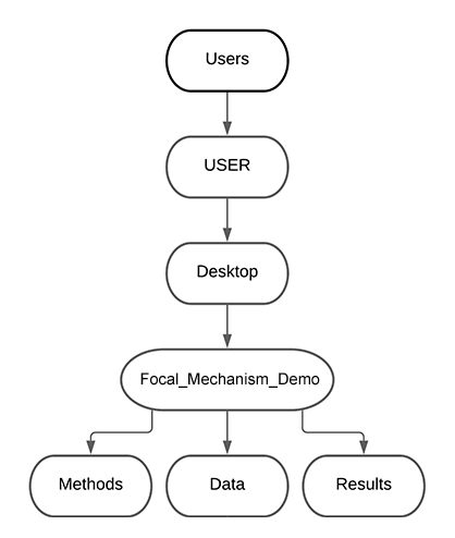
Created with Lucidchart
These folders can be created either by running the script provided below from anywhere after changing the main_dir file path to reflect your username or by manually creating a Focal_Mechanism_Demo folder and within it Data, Methods, and Results folders.
'''
Decription:
This script creates folders for the focal_mechanism_demo.py script if they don't already exist
'''

import os

# main directory path
main_dir = r'C:\Users\USER\Desktop\Focal_Mechanism_Demo'

# path to the directory holding the project data files
data_folder = os.path.join(main_dir, 'Data')

# path to the directory holding the project Python scripts
methods_folder = os.path.join(main_dir, 'Methods')

# path to the directory holding the map generated by the scripts
results_folder = os.path.join(main_dir, 'Results')

directories = [main_dir, data_folder, methods_folder, results_folder]

# Iterates through the list of directories and creates them if they don't already exist
for directory in directories:
    os.makedirs(directory, exist_ok = True)
Data files used and created by the demo script will be located in the Data folder, and the focal mechanism map will save to the Results folder. The Methods folder should contain the demo scripts.
Retrieve Focal Mechanism Data
Focal mechanism data will be acquired by downloading it from the SCEDC focal mechanism catalog. This demo uses the following search parameters:
Date range: 2019/01/01 to 2020/01/01 Magnitude range: 5 to 10 Latitude range: 35.5 to 36.1 Longitude range: -118 to -117.15 Depth range: -5 to 100
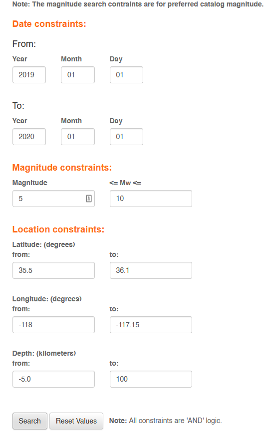
Example of entering the focal mechanism parameters into the Southern California Earthquake Data Center's focal mechanism catalog search
After clicking the search button, the results are presented as a text page. Select the data and column headers as shown below, and copy them into a text file. Then save the text file to the Data folder and name it focal_mechanism_data.
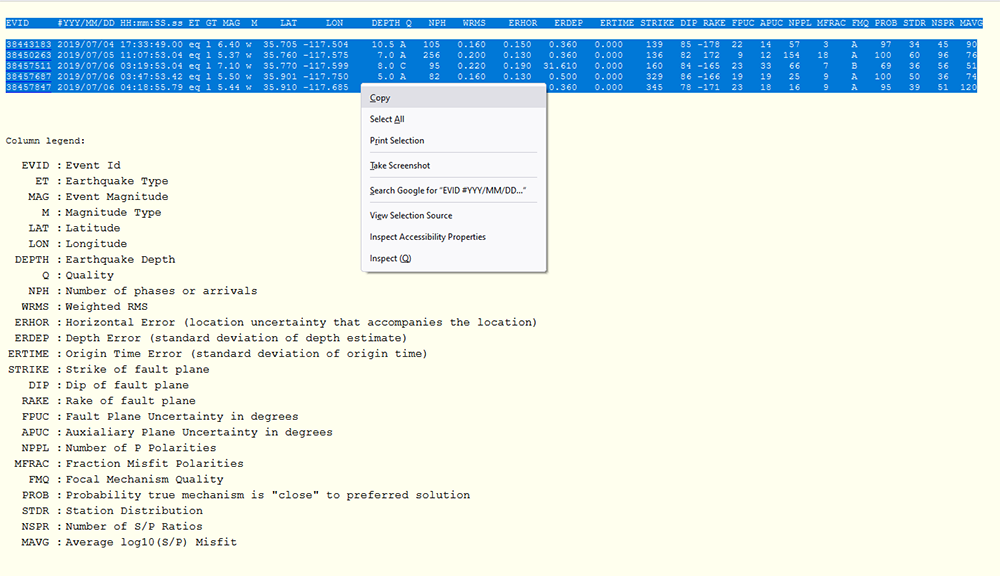
Example of selecting and copying the focal mechanism data and column headers
Creating The Project Files
Conditioning The Focal Mechanism Data
The focal mechanism data as retrieved from the SCEDC does not have a uniform delimiter separating the columns and has an empty line between the column header and the column values. In order to read the data into a data frame, it needs to be conditioned so that the aforementioned issues are resolved.
The following demo script function removes the empty line and standardizes the delimiter to be tabs, then saves the conditioned data as a CSV file:
    # Conditions focal mechanism files downloaded from the Southern California Earthquake Data Center so that they can be used
    def Condition_Focal_Mechanism_Data(self):
        import os
        import re

        print('Conditioning focal mechanisms...')


        input_file = os.path.join(self.main_dir, 'Data', 'focal_mechanism_data.txt')
        # reads in the file by line rather than the default of by character
        with open(input_file, 'r') as f:
            lines = f.readlines()

        # holds the conditioned lines, namely the removal of empty lines
        conditioned_lines = []
        # iterates over each line and adds them to a list as long as they are not empty
        for line in lines:
            if line == '\n':
                continue
            conditioned_lines.append(line)

        # empty placeholder for the conditioned lines list to be rejoined into a string
        conditioned_data = ''
        # rejoins the conditioned lines into a string so that it can be further conditioned
        conditioned_data = conditioned_data.join(conditioned_lines)

        # regular expression pattern for finding 1 or more white spaces (key) and the replacment value for matches (value)
        replacements = {' +':'\t'}
        # subsitutes text using the patterns in "replacements"
        for key, value in replacements.items():
            data = re.sub(key, value, conditioned_data)

        output_file = os.path.join(self.main_dir, 'Data', 'focal_mechanism_data.csv')
        with open(output_file, 'w') as f:
            f.write(data)
Filtering Focal Mechanism Data Into The “Aki” Format
After conditioning the focal mechanism data, it needs to be filtered so that the resulting file can be read by the PyGMT meca function, which plots focal mechanism “beach-balls.” As the data provided by the SCEDC is in terms of strike, drip, rake, and magnitude, the focal mechanism “beach-balls” will be determined by way of the Aki and Richards (1980) convention. In this demo, earthquakes greater than or equal to M7.0 will be offset to showcase how offsetting is accomplished. The meca function requires a file to be passed directly to the spec parameter when offsetting, so a CSV file with specific columns and column order pertaining to the convention needs to be created. Additionally, the column headers must be removed, so that header names don’t plot as text.
The following demo script function splits the focal mechanism data into two data frames at M7.0 earthquakes, then converts the magnitudes so that they are exponentially scaled; this is how the “beach-balls” will be sized when they are plotted. Next, it adds offset coordinates and text label columns to the data frame of M7.0 and greater earthquakes so they will be offset from their point of origin when plotted. Finally, the two data frames are saved as CSV files:
    # Creates a focal mechanism dataframe in the "aki" format from the focal mechanism data
    def Filter_AKI_Format_Focal_Mechanism_Data(self):
        import os
        import pandas as pd

        print('Writing focal mechanisms to CSV...')


        focal_mechanisms =  os.path.join(self.main_dir, 'Data', 'focal_mechanism_data.csv')
        df_focal_mechanisms = pd.read_csv(focal_mechanisms , sep='\t')

        # saves the unified depth column as a pandas series so that it can be recalled later for coloring the focal mechanisms by depth
        fm_depths = df_focal_mechanisms['DEPTH']
        # saves the unified depth magnitude column as a pandas series so that it can be recalled later for creating the legend
        fm_mags = df_focal_mechanisms['MAG']

        # magnitude of earthquakes used to filter out the focal mechanisms that will be offset
        magnitude_filter = 7

        # focal mechanisms with earthquake magnitude less than the magnitude filter
        df_mag_filtered_focal_mecha = df_focal_mechanisms[(df_focal_mechanisms.MAG < magnitude_filter)]
        # focal mechanisms with earthquake magnitude greater than or equal to the magnitude filter
        df_offset_mag_filtered_focal_mecha =df_focal_mechanisms[(df_focal_mechanisms.MAG >= magnitude_filter)]

        # reads the unmodifed magnitude of the focal mechanisms that will be offset into a list so it can be later used to label them
        fm_label = []
        for i in df_offset_mag_filtered_focal_mecha.MAG:
            fm_label.append(i)

        fm_dataframes = [df_mag_filtered_focal_mecha, df_offset_mag_filtered_focal_mecha]

        # iterates through each focal mechanism dataframe and scales them expoentially so that they will be plotted as exponentially larger sizes, and resets the index in place while not including the old index as a column which is done for tidyness
        for dataframe in fm_dataframes:
            dataframe.reset_index(inplace=True, drop=True)
            dataframe['MAG'] = 0.1 * (2 ** dataframe.MAG)

        # new dataframes to hold only the columns used for the "aki" focal mechanism format
        fm_aki_format = pd.DataFrame()
        fm_aki_format_offset = pd.DataFrame()
        aki_dataframes = [fm_aki_format, fm_aki_format_offset]
        # column names of the aki format, with keys being columns from the focal mechanism dataframes and values being the new column names to be used
        aki_format_attributes = {'LON':'longitude', 'LAT':'latitude', 'DEPTH':'depth', 'STRIKE':'strike', 'DIP':'dip', 'RAKE':'rake', 'MAG':'magnitude'}

        # add the desired columns for the 'aki' focal mechanism format to the new dataframes in the desired order
        for aki_data, fm_data in zip(aki_dataframes, fm_dataframes):
            for key, value in aki_format_attributes.items():
                aki_data[value] = fm_data[key]

        # offset coordinates (lon:lat) used for offsetting the selected focal mechanisms
        offset_coordinates = {-117.70:35.78}
        fm_aki_format_offset['offset_longitude'] = offset_coordinates.keys()
        fm_aki_format_offset['offset_latitude'] = offset_coordinates.values()

        # adds label data for plotting above each focal mechanism beachball
        fm_aki_format_offset['label_mag'] = fm_label

        # path to the "small" EQ focal mechanisms
        focal_mechanisms_lesser_output =  os.path.join(self.main_dir, 'Data', 'focal_mechanism_data_less_than_M{}.csv').format(magnitude_filter)
        # path to the "large" EQ focal mechanisms
        focal_mechanisms_greater_output =  os.path.join(self.main_dir, 'Data', 'focal_mechanism_data_greater_than_or_equal_to_M{}.csv').format(magnitude_filter)
        focal_mechanism_outputs = [focal_mechanisms_lesser_output, focal_mechanisms_greater_output]

        # writes the aki format dataframes to csv files, leaving out the header. This is important because if the header is included, fig.meca will plot the header text
        for dataframe, path in zip(aki_dataframes, focal_mechanism_outputs):
            dataframe.to_csv(path, sep='\t', index=False, header=None)

        return fm_depths, fm_mags, magnitude_filter
Creating The Legend
When the focal mechanisms “beach-balls” are eventually plotted on a map, the size differences will need to be given context with a legend. For this kind of legend, the PyGMT legend function needs to be passed a postscript file.
The following demo script function creates a postscript file for the legend:
# Creates a postscript legend file
def Create_Legend(self, fm_mags):
    import os
    import math

    # File path to postscript legend file to be created
    focal_mechanism_legend = os.path.join(self.main_dir, 'Data', 'focal_mechanism_legend.txt')

    # Creates a postscript file and writes some explainer, legend header text, and the column format
    with open(focal_mechanism_legend, 'w') as f:
        f.write(
            '# G is vertical gap, V is vertical line, N sets # of columns,\n'
            '# D draws horizontal line, H is header, L is column header,\n'
            '# S is symbol <symbol size><symbol color><symbol border thickness><text position><text>\n'
            '\n'
            'H 12p,Helvetica Magnitude\n'
            'D 0.1i 1p\n'
            'G 0.05i\n'
            'N 1\n'
            '\n'
        )

    # sets the index to the minimum magnitude of the unified dataset. This is used to set the minimum size for the circles used to represent magnitude within the legend, as well as label them
    i = math.floor(fm_mags.min())
    # sets the vertical space between each magnitude circle/text line
    v_spacer = 0.08

    # creteas a legend entry for each integer magnitude within the dataset and appends it to the legend file
    with open(focal_mechanism_legend, 'a') as f:
        while i <= round(fm_mags.max(), 0):\
            # replicates the exponential scaling of the magnitide and linear scaling of the fig.meca function so that the magnitude circles in the legend are the same size as the plotted focal mechanisms
            size = 0.1*(0.1*(2**i))
            size = round(size, 2)

            # creates a legend of transparent circles that are labeld with the associated magnitude
            f.write(
                'S 0.20i c {} white@100 0.5p 0.6i M{}\n'
                'G {}i\n'
                .format(size, i, v_spacer)
            )

            # exponentially scales the vertical spacing between each legend entry so that they are evenly spaced in this particular demo
            v_spacer = v_spacer**0.5
            i += 1
Building The Map
Now that the focal mechanism data and legend have been properly prepared, it’s time to plot everything on a map.
The following demo script function plots focal mechanism “beach-balls” over an automatically downloaded 3 arc second Digital Elevation Model from the Shuttle Radar Topography Mission. The “beach-balls” are scaled exponentially in size by the magnitude and colored by depth, with magnitude, and depth legends plotted along the map axes. An inset map displaying the study region relative to the greater region around it is plotted in the upper right corner of the map:
    # Plots the map
    def Plot_Map(self, fm_depths, magnitude_filter):
        import os
        import pygmt

        print('Building map...')

        ### BASEMAP -----------------------------------------------------------------------------
        # sets the region to be displayed in the map <min lon><max lon><min lat><max lat>
        region = [-118.0, -117.15, 35.5, 36.1]
        # map projection (Mercator): <type><size><units>
        projection = 'M6i'
        # frame  annotations: [<frame sides with/without ticks>, <x-axis tick rate>, <y-axis tick rate>]
        frame = ['SWne', 'xa', 'ya']
        # map scale - displays a fancy (f) distance scale (lScale) in kilometers (u). Format of <type><longitude><latitude>/<latitude of km symbol>/<scale length in km>+<unit>+<label><label text>
        map_scale = 'f-118.0/32.15/20/100+u+lScale:'


        ### GRID -----------------------------------------------------------------------------
        # sets the color palette table for the digital elevation map
        grid_cmap = 'grayC'


        ### MECA -----------------------------------------------------------------------------
        # focal mechanism data of earthquakes less than the magnitude filter
        focal_mechanisms_less_than_magnitude_filter = os.path.join(self.main_dir, 'Data', 'focal_mechanism_data_less_than_M{}.csv').format(magnitude_filter)
        # focal mechanism data of earthquakes greater than or equal to the magnitude filter
        focal_mechanisms_greater_than_magnitude_filter = os.path.join(self.main_dir, 'Data', 'focal_mechanism_data_greater_than_or_equal_to_M{}.csv').format(magnitude_filter)
        focal_mechanisms = [focal_mechanisms_less_than_magnitude_filter, focal_mechanisms_greater_than_magnitude_filter]
        # column format: <longitiude><latitude><strike><dip><rake><magnitude>. Optionally add <offset longitude><offset latitude><label> to the end
        convention = 'aki'
        # scale defines the size for magnitude = 5 (0.5). Also optionally plots labels above the focal mechanisms (+f15p,Helvetica,black).
        fm_scale = '0.5+f15p,Helvetica,black'
        # thickness of the lines drawn from the offset focal mechanisms back to their point of origin
        fm_offset = '1p'
        # colors by which to color focal mechanisms
        depth_color = 'yellow,red,purple'


        ### COLORBAR -----------------------------------------------------------------------------
        # automaticly determined fancy frame with label. Format of: <type>+<label><label text>
        cbar_frame = 'af+l"Depth (km)"'


        ### LEGENDS -----------------------------------------------------------------------------
        # path to the legend file
        legend = os.path.join(self.main_dir, 'Data', 'focal_mechanism_legend.txt')
        # <position>+<width>+<offset x-dir>/<offset y-dir>
        legend_position = 'JMR+w1.05i+o0.15i/-0.02i'
        # <background color>+<line thickness>
        #legend_box = '+gwhite+p1p'


        ### INSET MAP -----------------------------------------------------------------------------
        # extent of the inset map
        i_region = [-130, -105, 27, 45]
        i_projection = 'M1.75i'
        # sets the border types, line thickness, and color <border type><line thickness><color>. In this case 1 = national boundaries, 2 = state boundaries within America
        i_borders = ['1/0.8p,gray40', '2/0.8p,gray40']
        # sets the color of the land
        i_land = 'gray'
        # sets the shorline type, line thickness, and color <shoreline type><line thickness><line color>. In this case, 1 = coastline
        i_shorelines = '1/0.1p,gray40'
        i_pen = '1p,black'
        # sets the water color
        i_water = 'azure2'
        # shifts the inset map in the x-direction. Positive numbers shift up, negative numbers shifts down. <amount><units>
        i_xshift = '12.5c'
        # shifts the inset map in the y-direction. Positive numbers shift up, negative numbers shifts down. <amount><units>
        i_yshift ='11.0c'
        # first two list elements of 'rectangle' are the longitude and latitude of the bottom left corner of the rectangle, and the last two elements are the longitude and latitude of the uppper right corner.
        rectangle = [[region[0], region[2], region[1], region[3]]]
        # sets style of plot as rectagle (r) with first two list items as the longitude and latitude of the bottom left corner of the rectangle, and the last two list items as the longitude and latitude of the uppper right corner (+s)
        i_style = 'r+s'
        # sets an auto-detrmined frame with ticks in intervals of 10 (a10), then displays the frame with ticks on the top and right sides of the map (NE), but doesn't show ticks for the left and bottoms sides (sw)
        i_frame = ['a10', 'swNE']


        ### Save File -----------------------------------------------------------------------------
        # map save name
        save_name = os.path.join(self.main_dir, 'Results', 'Focal_Mechanism_Demo.png')
        # sets the transparency of the white space around the map
        save_transparency = False


        # Establishes a figure to hold map layers
        fig = pygmt.Figure()

        # Forces Lat/Lon to display as degree decimal
        pygmt.config(FORMAT_GEO_MAP = 'D')
        # Forces Lat/Lon to display with two decimal places <f>, as opposed the default that limits by significan digits <g>
        pygmt.config(FORMAT_FLOAT_OUT = '%.2f')
        # Forces the map frame annotation to be smaller
        pygmt.config(FONT_ANNOT_PRIMARY = '10p,Helvetica,black')
        # Forces the scale font to be smaller
        pygmt.config(FONT_LABEL = '10p,Helvetica,black')


        #  Basemap layer
        fig.basemap(
            region = region,
            projection = projection,
            frame = frame
        )


        # topography layer
        fig.grdimage(
            # downloads a 3 arc second shuttle radar topography mission digital elevation model of the region extent
            '@srtm_relief_03s',
            # applies shading to the grid
            shading = True,
            cmap = grid_cmap,
        )


        depth_series = [fm_depths.min(), fm_depths.max()]

        # makes a color palette table to color the events by depth
        pygmt.makecpt(
            cmap = depth_color,
            series = depth_series
        )

        for focal_mechanism in focal_mechanisms:

            fig.meca(
                # requires a file to be provided directly to the spec parameter if offseting the focal mechanisms is desired
                spec = focal_mechanism,
                # sets the focal mechanism convention
                convention = convention,
                # linear scaling factor with respect to M5 earthquakes
                scale = fm_scale,
                # sets the focal mechanisms to be colored by the previously created color palette table
                C = True,
                # controls whether to offset the focal mechanims
                offset = fm_offset,
            )


        # Plots the color bar for depth
        fig.colorbar(
            frame = cbar_frame
        )


        # plots the legend
        fig.legend(
            spec = legend,
            position = legend_position,
        )


        # plots the map scale
        fig.basemap(
            map_scale = map_scale
            )


        # Plots a mini coast map as an offset inset map
        fig.coast(
            region = i_region,
            projection = i_projection,
            frame = i_frame,
            land = i_land,
            borders = i_borders,
            shorelines = i_shorelines,
            water = i_water,
            xshift = i_xshift,
            yshift = i_yshift
        )

        # Plots a rectangle of the study area in the inset map
        fig.plot(
            data = rectangle,
            style = i_style,
            pen = i_pen,
            projection = i_projection
        )


        # Saves a copy of the generated figure
        fig.savefig(save_name, transparent = save_transparency)

        print('Map Saved!')
Result
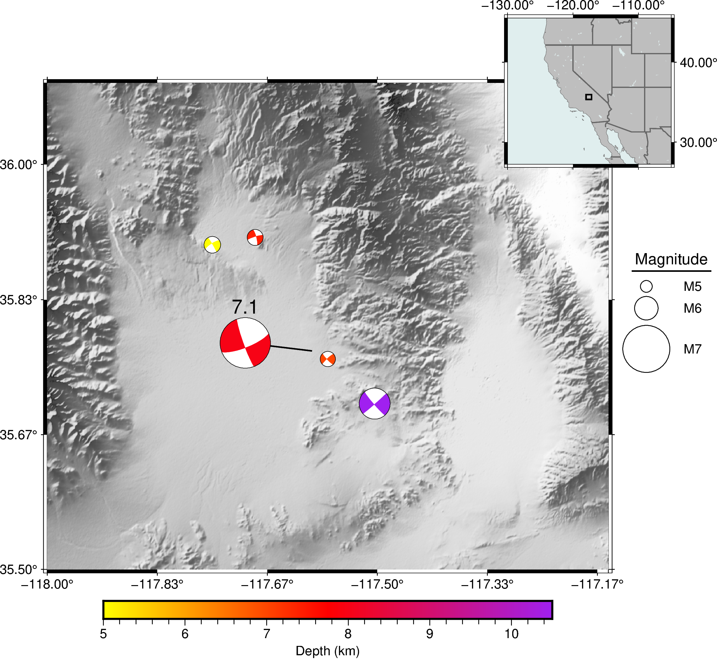
I hope that this has been helpful for anyone looking to plot and offset focal mechanisms with PyGMT.
Complete Code
'''
PyGMT v0.4.1

Decription:
This script creates a map of focal mechanisms that are scaled in size according to magnitude and colored according to depth.
It offsets selected focal mechanisms from their point of origin and draws a line to them.

Instructions:
1) Run the create_folder.py script to create the directory paths
2) Perform a focal mechanism search of the Souther California Earthquake Data Center focal mechanism catalog using the provided parameters
3) Copy the focal mechanism data and headers into a text file saved to the Data folder of this demo
4) Run this script

Focal Mechanism data source: https://service.scedc.caltech.edu/eq-catalogs/FMsearch.php

Date range: 2019/01/01 to 2020/01/01
Magnitude range: 5 to 10
Latitude range: 35.5 to 36.1
Longitude range: -118 to -117.15
Depth range: -5 to 100
'''

class Map_Builder():

    # Path to main project folder
    main_dir = r'C:\Users\USER\Desktop\Focal_Mechanism_Demo'


    # Conditions focal mechanism files downloaded from the Southern California Earthquake Data Center so that they can be used
    def Condition_Focal_Mechanism_Data(self):
        import os
        import re

        print('Conditioning focal mechanisms...')


        input_file = os.path.join(self.main_dir, 'Data', 'focal_mechanism_data.txt')
        # reads in the file by line rather than the default of by character
        with open(input_file, 'r') as f:
            lines = f.readlines()

        # holds the conditioned lines, namely the removal of empty lines
        conditioned_lines = []
        # iterates over each line and adds them to a list as long as they are not empty
        for line in lines:
            if line == '\n':
                continue
            conditioned_lines.append(line)

        # empty placeholder for the conditioned lines list to be rejoined into a string
        conditioned_data = ''
        # rejoins the conditioned lines into a string so that it can be further conditioned
        conditioned_data = conditioned_data.join(conditioned_lines)

        # regular expression pattern for finding 1 or more white spaces (key) and the replacment value for matches (value)
        replacements = {' +':'\t'}
        # subsitutes text using the patterns in "replacements"
        for key, value in replacements.items():
            data = re.sub(key, value, conditioned_data)

        output_file = os.path.join(self.main_dir, 'Data', 'focal_mechanism_data.csv')
        with open(output_file, 'w') as f:
            f.write(data)


    # Creates a focal mechanism dataframe in the "aki" format from the focal mechanism data
    def Filter_AKI_Format_Focal_Mechanism_Data(self):
        import os
        import pandas as pd

        print('Writing focal mechanisms to CSV...')


        focal_mechanisms =  os.path.join(self.main_dir, 'Data', 'focal_mechanism_data.csv')
        df_focal_mechanisms = pd.read_csv(focal_mechanisms , sep='\t')

        # saves the unified depth column as a pandas series so that it can be recalled later for coloring the focal mechanisms by depth
        fm_depths = df_focal_mechanisms['DEPTH']
        # saves the unified depth magnitude column as a pandas series so that it can be recalled later for creating the legend
        fm_mags = df_focal_mechanisms['MAG']

        # magnitude of earthquakes used to filter out the focal mechanisms that will be offset
        magnitude_filter = 7

        # focal mechanisms with earthquake magnitude less than the magnitude filter
        df_mag_filtered_focal_mecha = df_focal_mechanisms[(df_focal_mechanisms.MAG < magnitude_filter)]
        # focal mechanisms with earthquake magnitude greater than or equal to the magnitude filter
        df_offset_mag_filtered_focal_mecha =df_focal_mechanisms[(df_focal_mechanisms.MAG >= magnitude_filter)]

        # reads the unmodifed magnitude of the focal mechanisms that will be offset into a list so it can be later used to label them
        fm_label = []
        for i in df_offset_mag_filtered_focal_mecha.MAG:
            fm_label.append(i)

        fm_dataframes = [df_mag_filtered_focal_mecha, df_offset_mag_filtered_focal_mecha]

        # iterates through each focal mechanism dataframe and scales them expoentially so that they will be plotted as exponentially larger sizes, and resets the index in place while not including the old index as a column which is done for tidyness
        for dataframe in fm_dataframes:
            dataframe.reset_index(inplace=True, drop=True)
            dataframe['MAG'] = 0.1 * (2 ** dataframe.MAG)

        # new dataframes to hold only the columns used for the "aki" focal mechanism format
        fm_aki_format = pd.DataFrame()
        fm_aki_format_offset = pd.DataFrame()
        aki_dataframes = [fm_aki_format, fm_aki_format_offset]
        # column names of the aki format, with keys being columns from the focal mechanism dataframes and values being the new column names to be used
        aki_format_attributes = {'LON':'longitude', 'LAT':'latitude', 'DEPTH':'depth', 'STRIKE':'strike', 'DIP':'dip', 'RAKE':'rake', 'MAG':'magnitude'}

        # add the desired columns for the 'aki' focal mechanism format to the new dataframes in the desired order
        for aki_data, fm_data in zip(aki_dataframes, fm_dataframes):
            for key, value in aki_format_attributes.items():
                aki_data[value] = fm_data[key]

        # offset coordinates (lon:lat) used for offsetting the selected focal mechanisms
        offset_coordinates = {-117.70:35.78}
        fm_aki_format_offset['offset_longitude'] = offset_coordinates.keys()
        fm_aki_format_offset['offset_latitude'] = offset_coordinates.values()

        # adds label data for plotting above each focal mechanism beachball
        fm_aki_format_offset['label_mag'] = fm_label

        # path to the "small" EQ focal mechanisms
        focal_mechanisms_lesser_output =  os.path.join(self.main_dir, 'Data', 'focal_mechanism_data_less_than_M{}.csv').format(magnitude_filter)
        # path to the "large" EQ focal mechanisms
        focal_mechanisms_greater_output =  os.path.join(self.main_dir, 'Data', 'focal_mechanism_data_greater_than_or_equal_to_M{}.csv').format(magnitude_filter)
        focal_mechanism_outputs = [focal_mechanisms_lesser_output, focal_mechanisms_greater_output]

        # writes the aki format dataframes to csv files, leaving out the header. This is important because if the header is included, fig.meca will plot the header text
        for dataframe, path in zip(aki_dataframes, focal_mechanism_outputs):
            dataframe.to_csv(path, sep='\t', index=False, header=None)

        return fm_depths, fm_mags, magnitude_filter


    # Creates a postscript legend file
    def Create_Legend(self, fm_mags):
        import os
        import math

        # File path to postscript legend file to be created
        focal_mechanism_legend = os.path.join(self.main_dir, 'Data', 'focal_mechanism_legend.txt')

        # Creates a postscript file and writes some explainer, legend header text, and the column format
        with open(focal_mechanism_legend, 'w') as f:
            f.write(
                '# G is vertical gap, V is vertical line, N sets # of columns,\n'
                '# D draws horizontal line, H is header, L is column header,\n'
                '# S is symbol <symbol size><symbol color><symbol border thickness><text position><text>\n'
                '\n'
                'H 12p,Helvetica Magnitude\n'
                'D 0.1i 1p\n'
                'G 0.05i\n'
                'N 1\n'
                '\n'
            )

        # sets the index to the minimum magnitude of the unified dataset. This is used to set the minimum size for the circles used to represent magnitude within the legend, as well as label them
        i = math.floor(fm_mags.min())
        # sets the vertical space between each magnitude circle/text line
        v_spacer = 0.08

        # creteas a legend entry for each integer magnitude within the dataset and appends it to the legend file
        with open(focal_mechanism_legend, 'a') as f:
            while i <= round(fm_mags.max(), 0):\
                # replicates the exponential scaling of the magnitide and linear scaling of the fig.meca function so that the magnitude circles in the legend are the same size as the plotted focal mechanisms
                size = 0.1*(0.1*(2**i))
                size = round(size, 2)

                # creates a legend of transparent circles that are labeld with the associated magnitude
                f.write(
                    'S 0.20i c {} white@100 0.5p 0.6i M{}\n'
                    'G {}i\n'
                    .format(size, i, v_spacer)
                )

                # exponentially scales the vertical spacing between each legend entry so that they are evenly spaced in this particular demo
                v_spacer = v_spacer**0.5
                i += 1


    # Plots the map
    def Plot_Map(self, fm_depths, magnitude_filter):
        import os
        import pygmt

        print('Building map...')

        ### BASEMAP -----------------------------------------------------------------------------
        # sets the region to be displayed in the map <min lon><max lon><min lat><max lat>
        region = [-118.0, -117.15, 35.5, 36.1]
        # map projection (Mercator): <type><size><units>
        projection = 'M6i'
        # frame  annotations: [<frame sides with/without ticks>, <x-axis tick rate>, <y-axis tick rate>]
        frame = ['SWne', 'xa', 'ya']
        # map scale - displays a fancy (f) distance scale (lScale) in kilometers (u). Format of <type><longitude><latitude>/<latitude of km symbol>/<scale length in km>+<unit>+<label><label text>
        map_scale = 'f-118.0/32.15/20/100+u+lScale:'


        ### GRID -----------------------------------------------------------------------------
        # sets the color palette table for the digital elevation map
        grid_cmap = 'grayC'


        ### MECA -----------------------------------------------------------------------------
        # focal mechanism data of earthquakes less than the magnitude filter
        focal_mechanisms_less_than_magnitude_filter =  os.path.join(self.main_dir, 'Data', 'focal_mechanism_data_less_than_M{}.csv').format(magnitude_filter)
        # focal mechanism data of earthquakes greater than or equal to the magnitude filter
        focal_mechanisms_greater_than_magnitude_filter =  os.path.join(self.main_dir, 'Data', 'focal_mechanism_data_greater_than_or_equal_to_M{}.csv').format(magnitude_filter)
        focal_mechanisms = [focal_mechanisms_less_than_magnitude_filter, focal_mechanisms_greater_than_magnitude_filter]
        # column format: <longitiude><latitude><strike><dip><rake><magnitude>. Optionally add <offset longitude><offset latitude><label> to the end
        convention = 'aki'
        # scale defines the size for magnitude = 5 (0.5). Also optionally plots labels above the focal mechanisms (+f15p,Helvetica,black).
        fm_scale = '0.5+f15p,Helvetica,black'
        # thickness of the lines drawn from the offset focal mechanisms back to their point of origin
        fm_offset = '1p'
        # colors by which to color focal mechanisms
        depth_color = 'yellow,red,purple'


        ### COLORBAR -----------------------------------------------------------------------------
        # automaticly determined fancy frame with label. Format of: <type>+<label><label text>
        cbar_frame = 'af+l"Depth (km)"'


        ### LEGENDS -----------------------------------------------------------------------------
        # path to the legend file
        legend = os.path.join(self.main_dir, 'Data', 'focal_mechanism_legend.txt')
        # <position>+<width>+<offset x-dir>/<offset y-dir>
        legend_position = 'JMR+w1.05i+o0.15i/-0.02i'
        # <background color>+<line thickness>
        #legend_box = '+gwhite+p1p'


        ### INSET MAP -----------------------------------------------------------------------------
        # extent of the inset map
        i_region = [-130, -105, 27, 45]
        i_projection = 'M1.75i'
        # sets the border types, line thickness, and color <border type><line thickness><color>. In this case 1 = national boundaries, 2 = state boundaries within America
        i_borders = ['1/0.8p,gray40', '2/0.8p,gray40']
        # sets the color of the land
        i_land = 'gray'
        # sets the shorline type, line thickness, and color <shoreline type><line thickness><line color>. In this case, 1 = coastline
        i_shorelines = '1/0.1p,gray40'
        i_pen = '1p,black'
        # sets the water color
        i_water = 'azure2'
        # shifts the inset map in the x-direction. Positive numbers shift up, negative numbers shifts down. <amount><units>
        i_xshift = '12.5c'
        # shifts the inset map in the y-direction. Positive numbers shift up, negative numbers shifts down. <amount><units>
        i_yshift ='11.0c'
        # first two list elements of 'rectangle' are the longitude and latitude of the bottom left corner of the rectangle, and the last two elements are the longitude and latitude of the uppper right corner.
        rectangle = [[region[0], region[2], region[1], region[3]]]
        # sets style of plot as rectagle (r) with first two list items as the longitude and latitude of the bottom left corner of the rectangle, and the last two list items as the longitude and latitude of the uppper right corner (+s)
        i_style = 'r+s'
        # sets an auto-detrmined frame with ticks in intervals of 10 (a10), then displays the frame with ticks on the top and right sides of the map (NE), but doesn't show ticks for the left and bottoms sides (sw)
        i_frame = ['a10', 'swNE']


        ### Save File -----------------------------------------------------------------------------
        # map save name
        save_name = os.path.join(self.main_dir, 'Results', 'Focal_Mechanism_Demo.png')
        # sets the transparency of the white space around the map
        save_transparency = False


        # Establishes a figure to hold map layers
        fig = pygmt.Figure()

        # Forces Lat/Lon to display as degree decimal
        pygmt.config(FORMAT_GEO_MAP = 'D')
        # Forces Lat/Lon to display with two decimal places <f>, as opposed the default that limits by significan digits <g>
        pygmt.config(FORMAT_FLOAT_OUT = '%.2f')
        # Forces the map frame annotation to be smaller
        pygmt.config(FONT_ANNOT_PRIMARY = '10p,Helvetica,black')
        # Forces the scale font to be smaller
        pygmt.config(FONT_LABEL = '10p,Helvetica,black')


        #  Basemap layer
        fig.basemap(
            region = region,
            projection = projection,
            frame = frame
        )


        # topography layer
        fig.grdimage(
            # downloads a 3 arc second shuttle radar topography mission digital elevation model of the region extent
            '@srtm_relief_03s',
            # applies shading to the grid
            shading = True,
            cmap = grid_cmap,
        )


        depth_series = [fm_depths.min(), fm_depths.max()]

        # makes a color palette table to color the events by depth
        pygmt.makecpt(
            cmap = depth_color,
            series = depth_series
        )

        for focal_mechanism in focal_mechanisms:

            fig.meca(
                # requires a file to be provided directly to the spec parameter if offseting the focal mechanisms is desired
                spec = focal_mechanism,
                # sets the focal mechanism convention
                convention = convention,
                # linear scaling factor with respect to M5 earthquakes
                scale = fm_scale,
                # sets the focal mechanisms to be colored by the previously created color palette table
                C = True,
                # controls whether to offset the focal mechanims
                offset = fm_offset,
            )


        # Plots the color bar for depth
        fig.colorbar(
            frame = cbar_frame
        )


        # plots the legend
        fig.legend(
            spec = legend,
            position = legend_position,
        )


        # plots the map scale
        fig.basemap(
            map_scale = map_scale
            )


        # Plots a mini coast map as an offset inset map
        fig.coast(
            region = i_region,
            projection = i_projection,
            frame = i_frame,
            land = i_land,
            borders = i_borders,
            shorelines = i_shorelines,
            water = i_water,
            xshift = i_xshift,
            yshift = i_yshift
        )

        # Plots a rectangle of the study area in the inset map
        fig.plot(
            data = rectangle,
            style = i_style,
            pen = i_pen,
            projection = i_projection
        )


        # Saves a copy of the generated figure
        fig.savefig(save_name, transparent = save_transparency)

        print('Map Saved!')


data = Map_Builder()
data.Condition_Focal_Mechanism_Data()
fm_depths, fm_mags, magnitude_filter = data.Filter_AKI_Format_Focal_Mechanism_Data()
data.Create_Legend(fm_mags)
data.Plot_Map(fm_depths, magnitude_filter)Recommend
About Joyk
Aggregate valuable and interesting links.
Joyk means Joy of geeK