Source: https://unsplash.com/photos/OsYYPaPgIjw

Sales forecasting is one of the most common tasks that a data scientist has to face in daily business. In this article, I am going to use a Kaggle Competition dataset provided by one of the largest Russian Software companies.

In this competition, we are given sales for 34 months and are asked to predict total sales for every product and store in the next month. I have picked one single shop (shop_id =2) for simplicity to predict sales for this example.

With this Pandas code, we can select our shop and plot the monthly sales for the whole period:

We run that script and we can see these plots:

Sales per month. Source: AuthorBars plot of the same graph. Source: Author

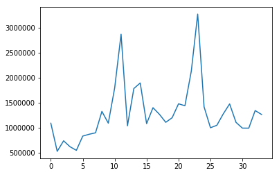
As we can see in the plots the sales volatility is quite large, with huge peaks and valleys in consecutive months.

The main technique used in time series forecasting is the ARIMA model and luckily Python offers a library with a lot of different options encompassing ARIMA models.

ARIMA stands for Autoregressive Integrated Moving Average and is a generalization of an autoregressive moving average (ARMA) model. Both of these models are fitted to time series, ARIMA models are applied in cases where data show evidence of non-stationarity, where an initial differencing step (corresponding to the “integrated” part of the model) can be applied one or more times to eliminate the non-stationarity. ARMA models are used when the data is stationary (not seasonal or not having trends).

The AR part of ARIMA indicates that the evolving variable of interest is regressed on its own lagged (i.e., prior) values. The MA part indicates that the regression error is actually a linear combination of error terms whose values occurred contemporaneously and at various times in the past. The I (for “integrated”) indicates that the data values have been replaced with the difference between their values and the previous values (and this differencing process may have been performed more than once). The purpose of each of these features is to make the model fit the data as well as possible.

As we can see in the official documentation, the form of the model is as follows:

model = sm.tsa.arima.ARIMA(target, order=(1, 0, 0))

The ARIMA function takes two variables, the target variable that we want to predict and the order. The order is made up of 3 different parameters: (p,d,q). Where p, d, and q are non-negative integers and:

• p is the order, the number of time lags, of the autoregressive model
• d is the degree of difference, that means, the number of times the data have had past values subtracted
• q is the order of the moving average model.

Now let’s implement a grid search function that will allow us to find the optimal values for our parameters. I will take the first 24 months as a train set and test the performance with MAE (minimum absolute error) in the following 10 months. Just like this:

When we run that code we can see the function returns this:

'the optimal (p,d,q) values are 9 with MAE:  57268.88088236949'

If we actually use those parameters we can plot our predictions against the real values:

That will return this plot:

Predictions vs Real values

We can see that the ARIMA model actually does a great job adjusting to our data, it obviously fits perfect the train data (months 0 to 24) but after that, it is completely impossible to fit all the swings in future months. Fortunately, the Kaggle competition only asks for a prediction for the one last month.

We can simplify our function to find the best parameters in case we want to predict only one month, doing this:

Now we obtain this when running the script:

the optimal (p,d,q) values are [2, 1, 3] with MAE:  219.79637413960882

As expected, the error is now much smaller.

So now that we know how to forecast time series using ARIMA, a question might come up immediately: why create a whole new method, i.e., time series (ARIMA), instead of using multiple linear regression and adding lagged variables to it?

Well, this is a very interesting topic. In fact, regression is the most used tool when forecasting, and one can actually fit a regression model to a time series, but there are several differences why this is not the best idea.

One immediate point is that a linear regression only works with observed variables while ARIMA incorporates unobserved variables in the moving average part; thus, ARIMA is more flexible.

AR model can be seen as a linear regression model and its coefficients can be estimated using Ordinary Least Squares: β^OLS=(X′X)−1X′yβ^OLS=(X′X)−1X′y where XX consists of lags of the dependent variable that are observed.

Meanwhile, MA or ARMA models do not fit into the OLS framework since some of the variables, namely the lagged error terms, are unobserved, and hence the OLS estimator is infeasible.

OK, that’s all for today, hope you enjoyed this article.

Happy coding!