Homotopy Type Theory

Erik Palmgren Memorial Conference

Erik Palmgren, 1963–2019

Erik Palmgren, professor of Mathematical Logic at Stockholm University, passed away unexpectedly in November 2019.

This conference will be an online workshop to remember and celebrate Erik’s life and work. There will be talks by Erik’s friends and colleagues, as well as time for discussions and exchange of memories during breaks. Talks may be about any topics that Erik would have enjoyed, including but not limited to (in Erik’s words):

– Type theory and its models. The relation between type theory and homotopy theory.
– Categorical logic and category-theoretic foundations.
– Constructive mathematics, especially formal topology and reverse constructive mathematics.
– Nonstandard analysis, especially its constructive aspects
– Philosophy of mathematics related to constructivism.

Online, 19–21 Nov 2020

http://logic.math.su.se/palmgren-memorial/

HoTT Dissertation Fellowship

Update (Nov. 13): Application deadline extended to December 1, 2020.

PhD students close to finishing their thesis are invited to apply for a Dissertation Fellowship in Homotopy Type Theory. This fellowship, generously funded by Cambridge Quantum Computing and Ilyas Khan, will provide $18,000 to support a graduate student finishing a dissertation on a topic broadly related to homotopy type theory. For instance, it can be used to fund a semester free from teaching duties, or to extend a PhD period by a few months.

Applications are due by November 15, 2020, with decisions to be announced in mid-December; the fellowship period can be any time between January 1, 2021 and June 30, 2022 at the discretion of the applicant. To apply, please send the following:

A research statement of no more than two pages, describing your thesis project and its relationship to homotopy type theory, when you are planning to finish your PhD, and what the money would be used for. Please also mention your current and past sources of support during your PhD, and say a little about your research plans post-graduation.
A current CV.
A letter from your advisor in support of your thesis plan, and confirming that your department will be able to use the money as planned.

The recipient of the fellowship will be selected by a committee consisting of Steve Awodey, Thierry Coquand, Emily Riehl, and Mike Shulman, and will be announced here.

Application materials should be submitted by email to: [email protected] .

The Cantor-Schröder-Bernstein Theorem for ∞-groupoids

The classical Cantor-Schröder-Bernstein Theorem (CSB) of set theory, formulated by Cantor and first proved by Bernstein, states that for any pair of sets, if there is an injection of each one into the other, then the two sets are in bijection.

There are proofs that use excluded middle but not choice. That excluded middle is absolutely necessary was recently established by Pierre Pradic and Chad E. Brown.

The appropriate principle of excluded middle for HoTT/UF says that every subsingleton (or proposition, or truth value) is either empty or pointed. The statement that every type is either empty or pointed is much stronger, and amounts to global choice, which is incompatible with univalence (Theorem 3.2.2 of the HoTT book). In fact, in the presence of global choice, every type is a set by Hedberg’s Theorem, but univalence gives types that are not sets. Excluded middle middle, however, is known to be compatible with univalence, and is validated in Voevodsky’s model of simplicial sets. And so is (non-global) choice, but we don’t need it here.

Can the Cantor-Schröder-Bernstein Theorem be generalized from sets to arbitrary homotopy types, or ∞-groupoids, in the presence of excluded middle? This seems rather unlikely at first sight:

CSB fails for 1-categories.
In fact, it already fails for posets. For example, the intervals $(0,1)$ and $[0,1]$ are order-embedded into each other, but they are not order isomorphic.
The known proofs of CSB for sets rely on deciding equality of elements of sets, but, in the presence of excluded middle, the types that have decidable equality are precisely the sets, by Hedberg’s Theorem.

In set theory, a map $f : X \to Y$ is an injection if and only if it is left-cancellable, in the sense that $f(x)=f(x')$ implies $x=x'$ . But, for types $X$ and $Y$ that are not sets, this notion is too weak, and, moreover, is not a proposition as the identity type $x = x'$ has multiple elements in general. The appropriate notion of embedding for a function $f$ of arbitrary types $X$ and $Y$ is given by any of the following two equivalent conditions:

The map $\mathrel{ap}(f,x,x') : x = x' \to f(x) = f(x')$ is an equivalence for any $x,x':X$ .
The fibers of $f$ are all subsingletons.

A map of sets is an embedding if and only if it is left-cancellable. However, for example, any map $1 \to Y$ that picks a point $y:Y$ is left-cancellable, but it is an embedding if and only if the point $y$ is homotopy isolated, which amounts to saying that the identity type $y = y$ is contractible. This fails, for instance, when the type $Y$ is the homotopical circle, for any point $y$ , or when $Y$ is a univalent universe and $y:Y$ is the two-point type, or any type with more than one automorphism.

It is the second characterization of embedding given above that we exploit here.

The Cantor-Schröder-Bernstein Theorem for homotopy types, or ∞-groupoids. For any two types, if each one is embedded into the other, then they are equivalent, in the presence of excluded middle.

We adapt Halmos’ proof in his book Naive Set Theory to our more general situation. We don’t need to invoke univalence, the existence of propositional truncations or any other higher inductive type for our construction. But we do rely on function extensionality.

Let $f : X \to Y$ and $g : Y \to X$ be embeddings of arbitrary types $X$ and $Y$ .

We say that $x:X$ is a $g$ -point if for any $x_0 : X$ and $n : \mathbb{N}$ with $(g \circ f)^n (x_0)=x$ , the $g$ -fiber of $x_0$ is inhabited. Using function extensionality and the assumption that $g$ is an embedding, we see that being a $g$ -point is property rather than data, because subsingletons are closed under products.

Considering $x_0=x$ and $n=0$ , we see that if $x$ is a $g$ -point then the $g$ -fiber of $x$ is inhabited, and hence we get a function $g^{-1}$ of $g$ -points of $X$ into $Y$ . By construction, we have that $g(g^{-1}(x))=x$ . In particular if $g(y)$ is a $g$ -point for a given $y:Y$ , we get $g(g^{-1}(g(y)))=g(y)$ , and because $g$ , being an embedding, is left-cancellable, we get
$g^{-1}(g(y))=y$ .

Now define $h:X \to Y$ by $h(x) = g^{-1}(x)$ if $x$ is a $g$ -point, and $h(x)=f(x)$ , otherwise.

To conclude the proof, it is enough to show that $h$ is left-cancellable and split-surjective, as any such map is an equivalence.

To see that $h$ is left-cancellable, it is enough to show that the images of $f$ and $g^{-1}$ in the definition of $h$ don’t overlap, because $f$ and $g^{-1}$ are left-cancellable. For that purpose, let $x$ be a non- $g$ -point and $x'$ be a $g$ -point, and, for the sake of contradiction, assume $f(x) = g^{-1}(x')$ . Then $g(f(x))=g(g^{-1}(x'))=x'$ . Now, because if $g(f(x))$ were a $g$ -point then so would be $x$ , we conclude that it isn’t, and hence neither is $x'$ , which contradicts the assumption.

To see that $h$ is a split surjection, say that $x : X$ is an $f$ -point if there are designated $x_0 : X$ and $n : \mathbb{N}$ with $(g \circ f)^n (x_0)=x$ and the $g$ -fiber of $x_0$ empty. This is data rather than property, and so this notion could not have been used for the construction of $h$ . But every non- $f$ -point is a $g$ -point, applying excluded middle to the $g$ -fiber of $x_0$ in the definition of $g$ -point.

Claim. If $g(y)$ is not a $g$ -point, then there is a designated point $(x : X , p : f(x)=y)$ of the $f$ -fiber of $y$ such that $x$ is not a $g$ -point either. To prove this, first notice that it is impossible that $g(y)$ is not an $f$ -point, by the above observation. But this is not enough to conclude that it is an $f$ -point, because excluded middle applies to subsingletons only, which the notion of $f$ -point isn’t. However, it is readily seen that if $g(y)$ is an $f$ -point, then there is a designated point $(x,p)$ in the $f$ -fiber of $y$ . From this it follows that it impossible that the subtype of the fiber consisting of the elements $(x,p)$ with $x$ not a $g$ -point is empty. But the $f$ -fiber of $y$ is a proposition because $f$ is an embedding, and hence so is the subtype, and therefore the claim follows by double-negation elimination.

We can now resume the proof that $h$ is a split surjection. For any $y:Y$ , we check whether or not $g(y)$ is a $g$ -point. If it is, we map $y$ to $g(y)$ , and if it isn’t we map $y$ to the point $x : X$ given by the claim.

This concludes the proof.

So, in this argument we don’t apply excluded middle to equality directly, which we wouldn’t be able to as the types $X$ and $Y$ are not necessarily sets. We instead apply it to (1) the property of being a $g$ -point, defined in terms of the fibers of $g$ , (2) a fiber of $g$ , and (3) a subtype of a fiber of $f$ . These three types are propositions because the functions $f$ and $g$ are embeddings rather than merely left-cancellable maps.

A version of this argument is available in Agda.

HoTT 2019 Last Call

Last call for submissions

INTERNATIONAL CONFERENCE AND SUMMER SCHOOL

ON HOMOTOPY TYPE THEORY

12-17 August 2019
Carnegie Mellon University, Pittsburgh USA

https://hott.github.io/HoTT-2019

Submission of talks and registration are open for the International
Homotopy Type Theory conference (HoTT 2019), to be held August 12-17,
2019, at Carnegie Mellon University in Pittsburgh, USA. Contributions
are welcome in all areas related to homotopy type theory, including
but not limited to:

* Homotopical and higher-categorical semantics of type theory
* Synthetic homotopy theory
* Applications of univalence and higher inductive types
* Cubical type theories and cubical models
* Formalization of mathematics and computer science in homotopy type
theory / univalent foundations

Please submit 1-paragraph abstracts through EasyChair here:

https://easychair.org/conferences/?conf=hott2019

The submission deadline is 1 June 2019; we expect to
notify accepted submissions by 15 June. This conference is run on the
“mathematics model”: full papers will not be submitted, submissions
will not be refereed, and submission is not a publication. Please
email [email protected] with any questions.

STUDENT PAPER AWARD

A prize of $500 (and distinguished billing in the conference program)
will be awarded to the best paper submitted by a student (or recently
graduated student). To be eligible, you must include in your
submission (or send separately to [email protected]) a link
to a preprint of your paper (e.g. on arXiv or a private web space).

REGISTRATION, ACCOMODATION, AND TRAVEL

Registration for the conference and the summer school is now open at
https://hott.github.io/HoTT-2019/registration/. A limited amount of
financial support is available for students and postdoctoral
researchers; application instructions are available at the web site,
as is information about accomodation and travel options.

INVITED SPEAKERS

Ulrik Buchholtz (TU Darmstadt, Germany)
Dan Licata (Wesleyan University, USA)
Andrew Pitts (University of Cambridge, UK)
Emily Riehl (Johns Hopkins University, USA)
Christian Sattler (University of Gothenburg, Sweden)
Karol Szumilo (University of Leeds, UK)

IMPORTANT DATES

Submission deadline: 1 June
Notification Date: 15 June
Final abstracts due: 1 July
Early Registration deadline: 1 July (reduced fee)
Late Registration deadline: 1 August (increased fee)
Conference: 12-17 August 2019

SUMMER SCHOOL

There will be an associated Homotopy Type Theory Summer School in
the preceding week, August 7th to 10th. The instructors and topics
will be:

Cubical methods: Anders Mortberg (Carnegie Mellon University, USA)
Formalization in Agda: Guillaume Brunerie (Stockholm University, Sweden)
Formalization in Coq: Kristina Sojakova (Cornell University, USA)
Higher topos theory: Mathieu Anel (Carnegie Mellon University, USA)
Semantics of type theory: Jonas Frey (Carnegie Mellon University, USA)
Synthetic homotopy theory: Egbert Rijke (University of Illinois, USA)

SCIENTIFIC COMMITTEE

Steve Awodey (Carnegie Mellon University, USA)
Andrej Bauer (University of Ljubljana, Slovenia)
Thierry Coquand (University of Gothenburg, Sweden)
Nicola Gambino (University of Leeds, UK)
Peter LeFanu Lumsdaine (Stockholm University, Sweden)
Michael Shulman (University of San Diego, USA), chair

We look forward to seeing you in Pittsburgh!

Introduction to Univalent Foundations of Mathematics with Agda

I am going to teach HoTT/UF with Agda at the Midlands Graduate School in April, and I produced lecture notes that I thought may be of wider use and so I am advertising them here.

The source files I used to generate the above html version of the notes are available at github, so that questions, issues and pull requests for fixes, improvements and feature requests are publicly available there.

Geometry in Modal HoTT now on Zoom

The workshop Geometry in Modal HoTT taking place next week at cmu will be available for online participation via Zoom! The recorded talks will be available on youtube (provided the speakers give their consent) sometime after the workshop.

HoTT 2019 Call for Submissions

Submissions of talks are now open for the International Homotopy Type Theory conference (HoTT 2019), to be held from August 12th to 17th, 2019, at Carnegie Mellon University in Pittsburgh, USA. Contributions are welcome in all areas related to homotopy type theory, including but not limited to:

Homotopical and higher-categorical semantics of type theory
Synthetic homotopy theory
Applications of univalence and higher inductive types
Cubical type theories and cubical models
Formalization of mathematics and computer science in homotopy type theory / univalent foundations

Please submit 1-paragraph abstracts through the EasyChair conference system here:

https://easychair.org/conferences/?conf=hott2019

The submission deadline is 1 April 2019; we expect to notify accepted submissions by 1 May. If you need an earlier decision for some reason (e.g. to apply for funding), please submit your abstract by 15 March and send an email to [email protected] notifying us that you need an early decision.

This conference is run on the “mathematics model” rather than the “computer science model”: full papers will not be submitted, submissions will not be refereed, and submission is not a publication (although a proceedings volume might be organized afterwards). More information, including registration, accomodation options, and travel, will be available as the conference approaches at the web site https://hott.github.io/HoTT-2019/ .

Please email [email protected] with any questions.

Cubical Agda

Last year I wrote a post about cubicaltt on this blog. Since then there have been a lot of exciting developments in the world of cubes. In particular there are now two cubical proof assistants that are currently being developed in Gothenburg and Pittsburgh. One of them is a cubical version of Agda developed by Andrea Vezzosi at Chalmers and the other is a system called redtt developed by my colleagues at CMU.

These systems differ from cubicaltt in that they are proper proof assistants for cubical type theory in the sense that they support unification, interactive proof development via holes, etc… Cubical Agda inherits Agda’s powerful dependent pattern matching functionality, and redtt has a succinct notation for defining functions by eliminators. Our goal with cubicaltt was never to develop yet another proof assistant, but rather to explore how it could be to program and work in a core system based on cubical type theory. This meant that many things were quite tedious to do in cubicaltt, so it is great that we now have these more advanced systems that are much more pleasant to work in.

This post is about Cubical Agda, but more or less everything in it can also be done (with slight modifications) in redtt. This extension of Agda has actually been around for a few years now, however it is just this year that the theory of HITs has been properly worked out for cubical type theory:

On Higher Inductive Types in Cubical Type Theory

Inspired by this paper (which I will refer as “CHM”) Andrea has extended Cubical Agda with user definable HITs with definitional computation rules for all constructors. Working with these is a lot of fun and I have been doing many of the proofs in synthetic homotopy theory from the HoTT book cubically. Having a system with native support for HITs makes many things a lot easier and most of the proofs I have done are significantly shorter. However, this post will not focus on HITs, but rather on a core library for Cubical Agda that we have been developing over the last few months:

https://github.com/agda/cubical

The core part of this library has been designed with the aim to:

1. Expose and document the cubical primitives of Agda.

2. Provide an interface to HoTT as presented in the book (i.e. “Book HoTT”), but where everything is implemented with the cubical primitives under the hood.

The idea behind the second of these was suggested to me by Martín Escardó who wanted a file which exposes an identity type with the standard introduction principle and eliminator (satisfying the computation rule definitionally), together with function extensionality, univalence and propositional truncation. All of these notions should be represented using cubical primitives under the hood which means that they all compute and that there are no axioms involved. In particular this means that one can import this file in an Agda developments relying on Book HoTT and no axioms should then be needed; more about this later.

Our cubical library compiles with the latest development version of Agda and it is currently divided into 3 main parts:

Cubical.Basics

Cubical.Core

Cubical.HITs

The first of these contain various basic results from HoTT/UF, like isomorphisms are equivalences (i.e. have contractible fibers), Hedberg’s theorem (types with decidable equality are sets), various proofs of different formulations of univalence, etc. This part of the library is currently in flux as I’m adding a lot of results to it all the time.

The second one is the one I will focus on in this post and it is supposed to be quite stable by now. The files in this folder expose the cubical primitives and the cubical interface to HoTT/UF. Ideally a regular user should not have to look too closely at these files and instead just import Cubical.Core.Everything or Cubical.Core.HoTT-UF.

The third folder contains various HITs (S¹, S², S³, torus, suspension, pushouts, interval, join, smash products…) with some basic theory about these. I plan to write another post about this soon, so stay tuned.

As I said above a regular user should only really need to know about the Cubical.Core.Everything and Cubical.Core.HoTT-UF files in the core library. The Cubical.Core.Everything file exports the following things:

-- Basic primitives (some are from Agda.Primitive)

open import Cubical.Core.Primitives public

-- Basic cubical prelude

open import Cubical.Core.Prelude public

-- Definition of equivalences, Glue types and

-- the univalence theorem

open import Cubical.Core.Glue public

-- Propositional truncation defined as a

-- higher inductive type

open import Cubical.Core.PropositionalTruncation public

-- Definition of Identity types and definitions of J,

-- funExt, univalence and propositional truncation

-- using Id instead of Path

open import Cubical.Core.Id public

I will explain the contents of the Cubical.Core.HoTT-UF file in detail later in this post, but I would first like to clarify that it is absolutely not necessary to use that file as a new user. The point of it is mainly to provide a way to make already existing HoTT/UF developments in Agda compute, but I personally only use the cubical primitives provided by the Cubical.Core.Everything file when developing something new in Cubical Agda as I find these much more natural to work with (especially when reasoning about HITs).

Cubical Primitives

It is not my intention to write another detailed explanation of cubical type theory in this post; for that see my previous post and the paper (which is commonly referred to as “CCHM”, after the authors of CCHM):

Cubical Type Theory: a constructive interpretation of the univalence axiom

The main things that the CCHM cubical type theory extends dependent type theory with are:

An interval pretype
Kan operations
Glue types
Cubical identity types

The first of these is what lets us work directly with higher dimensional cubes in type theory and incorporating this into the judgmental structure is really what makes the system tick. The Cubical.Core.Primitives and Cubical.Core.Prelude files provide 1 and 2, together with some extra stuff that are needed to get 3 and 4 up and running.

Let’s first look at the cubical interval I. It has endpoints i0 : I and i1 : I together with connections and reversals:

_∧_ : I → I → I

_∨_ : I → I → I

~_ : I → I

satisfying the structure of a De Morgan algebra (as in CCHM). As Agda doesn’t have a notion of non-fibrant types (yet?) the interval I lives in Setω.

There are also (dependent) cubical Path types:

PathP : ∀ {ℓ} (A : I → Set ℓ) → A i0 → A i1 → Set ℓ

from which we can define non-dependent Paths:

Path : ∀ {ℓ} (A : Set ℓ) → A → A → Set ℓ

Path A a b = PathP (λ _ → A) a b

A non-dependent path Path A a b gets printed as a ≡ b. I would like to generalize this at some point and have cubical extension types (inspired by A type theory for synthetic ∞-categories). These extension types are already in redtt and has proved to be very natural and useful, especially for working with HITs as shown by this snippet of redtt code coming from the proof that the loop space of the circle is the integers:

def decode-square

: (n : int)

→ [i j] s1 [

| i=0 → loopn (pred n) j

| i=1 → loopn n j

| j=0 → base

| j=1 → loop i

]

= ...

Just like in cubicaltt we get short proofs of the basic primitives from HoTT/UF:

refl : ∀ {ℓ} {A : Set ℓ} (x : A) → x ≡ x

refl x = λ _ → x

sym : ∀ {ℓ} {A : Set ℓ} {x y : A} → x ≡ y → y ≡ x

sym p = λ i → p (~ i)

cong : ∀ {ℓ ℓ'} {A : Set ℓ} {B : A → Set ℓ'} {x y : A}

(f : (a : A) → B a)

(p : x ≡ y) →

PathP (λ i → B (p i)) (f x) (f y)

cong f p = λ i → f (p i)

funExt : ∀ {ℓ ℓ'} {A : Set ℓ} {B : A → Set ℓ'}

{f g : (x : A) → B x}

(p : (x : A) → f x ≡ g x) →

f ≡ g

funExt p i x = p x i

Note that the proof of functional extensionality is just swapping the arguments to p!

Partial elements and cubical subtypes

[In order for me to be able to explain the other features of Cubical Agda in some detail I have to spend some time on partial elements and cubical subtypes, but as these notions are quite technical I would recommend readers who are not already familiar with them to just skim over this section and read it more carefully later.]

One of the key operations in the cubical set model is to map an element of the interval to an element of the face lattice (i.e. the type of cofibrant propositions F ⊂ Ω). This map is written (_ = 1) : I → F in CCHM and in Cubical Agda it is written IsOne r. The constant 1=1 is a proof that (i1 = 1), i.e. of IsOne i1.

This lets us then work with partial types and elements directly (which was not possible in cubicaltt). The type Partial φ A is a special version of the function space IsOne φ → A with a more extensional judgmental equality. There is also a dependent version PartialP φ A which allows A to be defined only on φ. As these types are not necessarily fibrant they also live in Setω. These types are easiest to understand by seeing how one can introduce them:

sys : ∀ i → Partial (i ∨ ~ i) Set₁

sys i (i = i1) = Set → Set

sys i (i = i0) = Set

This defines a partial type in Set₁ which is defined when (i = i1) ∨ (i = i0). We define it by pattern matching so that it is Set → Set when (i = i1) and Set when (i = i0). Note that we are writing (i ∨ ~ i) and that the IsOne map is implicit. If one instead puts a hole as right hand side:

sys : ∀ i → Partial (i ∨ ~ i) Set₁

sys i x = {! x !}

and ask Agda what the type of x is (by putting the cursor in the hole and typing C-c C-,) then Agda answers:

Goal: Set₁

—————————————————————————————————————————————

x : IsOne (i ∨ ~ i)

i : I

I usually introduce these using pattern matching lambdas so that I can write:

sys' : ∀ i → Partial (i ∨ ~ i) Set₁

sys' i = \ { (i = i0) → Set

; (i = i1) → Set → Set }

This is very convenient when using the Kan operations. Furthermore, when the cases overlap they must of course agree:

sys2 : ∀ i j → Partial (i ∨ (i ∧ j)) Set₁

sys2 i j = \ { (i = i1) → Set

; (i = i1) (j = i1) → Set }

In order to get this to work Andrea had to adapt the pattern-matching of Agda to allow us to pattern-match on the faces like this. It is however not yet possible to use C-c C-c to automatically generate the cases for a partial element, but hopefully this will be added at some point.

Using the partial elements there are also cubical subtypes as in CCHM:

_[_↦_] : ∀ {ℓ} (A : Set ℓ) (φ : I) (u : Partial φ A) →

Agda.Primitive.Setω

A [ φ ↦ u ] = Sub A φ u

So that a : A [ φ ↦ u ] is a partial element a : A that agrees with u on φ. We have maps in and out of the subtypes:

inc : ∀ {ℓ} {A : Set ℓ} {φ} (u : A) →

A [ φ ↦ (λ _ → u) ]

ouc : ∀ {ℓ} {A : Set ℓ} {φ : I} {u : Partial φ A} →

A [ φ ↦ u ] → A

It would be very nice to have subtyping for these, but at the moment the user has to write inc/ouc explicitly. With this infrastructure we can now consider the Kan operations of cubical type theory.

Kan operations

In order to support HITs we use the Kan operations from CHM. The first of these is a generalized transport operation:

transp : ∀ {ℓ} (A : I → Set ℓ) (φ : I) (a : A i0) → A i1

When calling transp A φ a Agda makes sure that A is constant on φ and when calling this with i0 for φ we recover the regular transport function, furthermore when φ is i1 this is the identity function. Being able to control when transport is the identity function is really what makes this operation so useful (see the definition of comp below) and why we got HITs to work so nicely in CHM compared to CCHM.

We also have homogeneous composition operations:

hcomp : ∀ {ℓ} {A : Set ℓ} {φ : I}

(u : I → Partial A φ) (a : A) → A

When calling hcomp A φ u a Agda makes sure that a agrees with u i0 on φ. This is like the composition operations in CCHM, but the type A is constant. Note that this operation is actually different from the one in CHM as φ is in the interval and not the face lattice. By the way the partial elements are set up the faces will then be compared under the image of IsOne. This subtle detail is actually very useful and gives a very neat trick for eliminating empty systems from Cubical Agda (this has not yet been implemented, but it is discussed here).

Using these two operations we can derive the heterogeneous composition
operation:

comp : ∀ {ℓ : I → Level} (A : ∀ i → Set (ℓ i)) {φ : I}

(u : ∀ i → Partial φ (A i))

(u0 : A i0 [ φ ↦ u i0 ]) → A i1

comp A {φ = φ} u u0 =

hcomp

(λ i → λ { (φ = i1) →

transp (λ j → A (i ∨ j)) i (u _ 1=1) })

(transp A i0 (ouc u0))

This decomposition of the Kan operations into transport and homogeneous composition seems crucial to get HITs to work properly in cubical type theory and in fact redtt is also using a similar decomposition of their Kan operations.

We can also derive both homogeneous and heterogeneous Kan filling using hcomp and comp with connections:

hfill : ∀ {ℓ} {A : Set ℓ} {φ : I}

(u : ∀ i → Partial φ A)

(u0 : A [ φ ↦ u i0 ])

(i : I) → A

hfill {φ = φ} u u0 i =

hcomp (λ j → λ { (φ = i1) → u (i ∧ j) 1=1

; (i = i0) → ouc u0 })

(ouc u0)

fill : ∀ {ℓ : I → Level} (A : ∀ i → Set (ℓ i)) {φ : I}

(u : ∀ i → Partial φ (A i))

(u0 : A i0 [ φ ↦ u i0 ])

(i : I) → A i

fill A {φ = φ} u u0 i =

comp (λ j → A (i ∧ j))

(λ j → λ { (φ = i1) → u (i ∧ j) 1=1

; (i = i0) → ouc u0 })

(inc {φ = φ ∨ (~ i)} (ouc {φ = φ} u0))

Using these operations we can do all of the standard cubical stuff, like composing paths and defining J with its computation rule (up to a Path):

compPath : ∀ {ℓ} {A : Set ℓ} {x y z : A} →

x ≡ y → y ≡ z → x ≡ z

compPath {x = x} p q i =

hcomp (λ j → \ { (i = i0) → x

; (i = i1) → q j })

(p i)

module _ {ℓ ℓ'} {A : Set ℓ} {x : A}

(P : ∀ y → x ≡ y → Set ℓ') (d : P x refl) where

J : {y : A} → (p : x ≡ y) → P y p

J p = transp (λ i → P (p i) (λ j → p (i ∧ j))) i0 d

JRefl : J refl ≡ d

JRefl i = transp (λ _ → P x refl) i d

The use of a module here is not crucial in any way, it’s just an Agda trick to make J and JRefl share some arguments.

Glue types and univalence

The file Cubical.Core.Glue defines fibers and equivalences (as they were originally defined by Voevodsky in his Foundations library, i.e. as maps with contractible fibers). Using this we export the Glue types of Cubical Agda which lets us extend a total type by a partial family of equivalent types:

Glue : ∀ {ℓ ℓ'} (A : Set ℓ) {φ : I} →

(Te : Partial φ (Σ[ T ∈ Set ℓ' ] T ≃ A)) →

Set ℓ'

This comes with introduction and elimination forms (glue and unglue). With this we formalize the proof of a variation of univalence following the proof in Section 7.2 of CCHM. The key observation is that unglue is an equivalence:

unglueIsEquiv : ∀ {ℓ} (A : Set ℓ) (φ : I)

(f : PartialP φ (λ o → Σ[ T ∈ Set ℓ ] T ≃ A)) →

isEquiv {A = Glue A f} (unglue {φ = φ})

equiv-proof (unglueIsEquiv A φ f) = λ (b : A) →

let u : I → Partial φ A

u i = λ{ (φ = i1) → equivCtr (f 1=1 .snd) b .snd (~ i) }

ctr : fiber (unglue {φ = φ}) b

ctr = ( glue (λ { (φ = i1) → equivCtr (f 1=1 .snd) b .fst }) (hcomp u b)

, λ j → hfill u (inc b) (~ j))

in ( ctr

, λ (v : fiber (unglue {φ = φ}) b) i →

let u' : I → Partial (φ ∨ ~ i ∨ i) A

u' j = λ { (φ = i1) → equivCtrPath (f 1=1 .snd) b v i .snd (~ j)

; (i = i0) → hfill u (inc b) j

; (i = i1) → v .snd (~ j) }

in ( glue (λ { (φ = i1) → equivCtrPath (f 1=1 .snd) b v i .fst }) (hcomp u' b)

, λ j → hfill u' (inc b) (~ j)))

The details of this proof is best studied interactively in Agda and by first understanding the proof in CCHM. The reason this is a crucial observation is that it says that any partial family of equivalences can be extended to a total one from Glue [ φ ↦ (T,f) ] A to A:

unglueEquiv : ∀ {ℓ} (A : Set ℓ) (φ : I)

(f : PartialP φ (λ o → Σ[ T ∈ Set ℓ ] T ≃ A)) →

(Glue A f) ≃ A

unglueEquiv A φ f = ( unglue {φ = φ} , unglueIsEquiv A φ f )

and this is exactly what we need to prove the following formulation of the univalence theorem:

EquivContr : ∀ {ℓ} (A : Set ℓ) → isContr (Σ[ T ∈ Set ℓ ] T ≃ A)

EquivContr {ℓ} A =

( ( A , idEquiv A)

, λ w i →

let f : PartialP (~ i ∨ i) (λ x → Σ[ T ∈ Set ℓ ] T ≃ A)

f = λ { (i = i0) → ( A , idEquiv A ) ; (i = i1) → w }

in ( Glue A f , unglueEquiv A (~ i ∨ i) f) )

This formulation of univalence was proposed by Martín Escardó in (see also Theorem 5.8.4 of the HoTT Book):

https://groups.google.com/forum/#!msg/homotopytypetheory/HfCB_b-PNEU/Ibb48LvUMeUJ

We have also formalized a quite slick proof of the standard formulation of univalence from EquivContr (see Cubical.Basics.Univalence). This proof uses that EquivContr is contractibility of singletons for equivalences, which combined with subst can be used to prove equivalence induction:

contrSinglEquiv : ∀ {ℓ} {A B : Set ℓ} (e : A ≃ B) →

(B , idEquiv B) ≡ (A , e)

contrSinglEquiv {A = A} {B = B} e =

isContr→isProp (EquivContr B) (B , idEquiv B) (A , e)

EquivJ : ∀ {ℓ ℓ′} (P : (A B : Set ℓ) → (e : B ≃ A) → Set ℓ′)

(r : (A : Set ℓ) → P A A (idEquiv A))

(A B : Set ℓ) (e : B ≃ A) →

P A B e

EquivJ P r A B e =

subst (λ x → P A (x .fst) (x .snd))

(contrSinglEquiv e) (r A)

We then use that the Glue types also gives a map ua which maps the identity equivalence to refl:

ua : ∀ {ℓ} {A B : Set ℓ} → A ≃ B → A ≡ B

ua {A = A} {B = B} e i =

Glue B (λ { (i = i0) → (A , e)

; (i = i1) → (B , idEquiv B) })

uaIdEquiv : ∀ {ℓ} {A : Set ℓ} → ua (idEquiv A) ≡ refl

uaIdEquiv {A = A} i j =

Glue A {φ = i ∨ ~ j ∨ j} (λ _ → A , idEquiv A)

Now, given any function au : ∀ {ℓ} {A B : Set ℓ} → A ≡ B → A ≃ B satisfying auid : ∀ {ℓ} {A B : Set ℓ} → au refl ≡ idEquiv A we directly get that this is an equivalence using the fact that any isomorphism is an equivalence:

module Univalence

(au : ∀ {ℓ} {A B : Set ℓ} → A ≡ B → A ≃ B)

(auid : ∀ {ℓ} {A B : Set ℓ} → au refl ≡ idEquiv A) where

thm : ∀ {ℓ} {A B : Set ℓ} → isEquiv au

thm {A = A} {B = B} =

isoToIsEquiv {B = A ≃ B} au ua

(EquivJ (λ _ _ e → au (ua e) ≡ e)

(λ X → compPath (cong au uaIdEquiv)

(auid {B = B})) _ _)

(J (λ X p → ua (au p) ≡ p)

(compPath (cong ua (auid {B = B})) uaIdEquiv))

We can then instantiate this with for example the au map defined using J (which is how Vladimir originally stated the univalence axiom):

eqweqmap : ∀ {ℓ} {A B : Set ℓ} → A ≡ B → A ≃ B

eqweqmap {A = A} e = J (λ X _ → A ≃ X) (idEquiv A) e

eqweqmapid : ∀ {ℓ} {A : Set ℓ} → eqweqmap refl ≡ idEquiv A

eqweqmapid {A = A} = JRefl (λ X _ → A ≃ X) (idEquiv A)

univalenceStatement : ∀ {ℓ} {A B : Set ℓ} →

isEquiv (eqweqmap {ℓ} {A} {B})

univalenceStatement = Univalence.thm eqweqmap eqweqmapid

Note that eqweqmapid is not proved by refl, instead we need to use the fact that the computation rule for J holds up to a Path. Furthermore, I would like to emphasize that there is no problem with using J for Path’s and that the fact that the computation rule doesn’t hold definitionally is almost never a problem for practical formalization as one rarely use it as it is often more natural to just use the cubical primitives. However, in Section 9.1 of CCHM we solve this by defining cubical identity types satisfying the computation rule definitionally (following a trick of Andrew Swan).

Cubical identity types

The idea behind the cubical identity types is that an element of an identity type is a pair of a path and a formula which tells us where this path is constant, so for example reflexivity is just the constant path together with the fact that it is constant everywhere (note that the interval variable comes before the path as the path depends on it):

refl : ∀ {ℓ} {A : Set ℓ} {x : A} → Id x x

refl {x = x} = ⟨ i1 , (λ _ → x) ⟩

These types also come with an eliminator from which we can prove J such that it is the identity function on refl, i.e. where the computation rule holds definitionally (for details see the Agda code in Cubical.Core.Id). We then prove that Path and Id are equivalent types and develop the theory that we have for Path for Id as well, in particular we prove the univalence theorem expressed with Id everywhere (the usual formulation can be found in Cubical.Basics.UnivalenceId).

Note that the cubical identity types are not an inductive family like in HoTT which means that we cannot use Agda’s pattern-matching to match on them. Furthermore Cubical Agda doesn’t support inductive families yet, but it should be possible to adapt the techniques of Cavallo/Harper presented in

Higher Inductive Types in Cubical Computational Type Theory

in order to extend it with inductive families. The traditional identity types could then be defined as in HoTT and pattern-matching should work as expected.

Propositional truncation

The core library only contains one HIT: propositional truncation (Cubical.Core.PropositionalTruncation). As Cubical Agda has native support for user defined HITs this is very convenient to define:

data ∥_∥ {ℓ} (A : Set ℓ) : Set ℓ where

∣_∣ : A → ∥ A ∥

squash : ∀ (x y : ∥ A ∥) → x ≡ y

We can then prove the recursor (and eliminator) using pattern-matching:

recPropTrunc : ∀ {ℓ} {A : Set ℓ} {P : Set ℓ} →

isProp P → (A → P) → ∥ A ∥ → P

recPropTrunc Pprop f ∣ x ∣ = f x

recPropTrunc Pprop f (squash x y i) =

Pprop (recPropTrunc Pprop f x) (recPropTrunc Pprop f y) i

However I would not only use recPropTrunc explicitly as we can just use pattern-matching to define functions out of HITs. Note that the cubical machinery makes it possible for us to define these pattern-matching equations in a very nice way without any ap‘s. This is one of the main reasons why I find it a lot more natural to work with HITs in cubical type theory than in Book HoTT: the higher constructors of HITs construct actual elements of the HIT, not of its identity type!

This is just a short example of what can be done with HITs in Cubical Agda, I plan to write more about this in a future post, but for now one can look at the folder Cubical/HITs for many more examples (S¹, S², S³, torus, suspension, pushouts, interval, join, smash products…).

Constructive HoTT/UF

By combining everything I have said so far we have written the file Cubical.Core.HoTT-UF which exports the primitives of HoTT/UF defined using cubical machinery under the hood:

open import Cubical.Core.Id public

using ( _≡_ -- The identity type.

; refl -- Unfortunately, pattern matching on refl is not available.

; J -- Until it is, you have to use the induction principle J.

; transport -- As in the HoTT Book.

; ap

; _∙_

; _⁻¹

; _≡⟨_⟩_ -- Standard equational reasoning.

; _∎

; funExt -- Function extensionality

-- (can also be derived from univalence).

; Σ -- Sum type. Needed to define contractible types, equivalences

; _,_ -- and univalence.

; pr₁ -- The eta rule is available.

; pr₂

; isProp -- The usual notions of proposition, contractible type, set.

; isContr

; isSet

; isEquiv -- A map with contractible fibers

-- (Voevodsky's version of the notion).

; _≃_ -- The type of equivalences between two given types.

; EquivContr -- A formulation of univalence.

; ∥_∥ -- Propositional truncation.

; ∣_∣ -- Map into the propositional truncation.

; ∥∥-isProp -- A truncated type is a proposition.

; ∥∥-recursion -- Non-dependent elimination.

; ∥∥-induction -- Dependent elimination.

)

The idea is that if someone has some code written using HoTT/UF axioms in Agda they can just import this file and everything should compute properly. The only downside is that one has to rewrite all pattern-matches on Id to explicit uses of J, but if someone is willing to do this and have some cool examples that now compute please let me know!

That’s all I had to say about the library for now. Pull-requests and feedback on how to improve it are very welcome! Please use the Github page for the library for comments and issues:

https://github.com/agda/cubical/issues

If you find some bugs in Cubical Agda you can use the Github page of Agda to report them (just check that no-one has already reported the bug):

https://github.com/agda/agda/issues

Impredicative Encodings, Part 3

In this post I will argue that, improving on previous work of Awodey-Frey-Speight, (higher) inductive types can be defined using impredicative encodings with their full dependent induction principles — in particular, eliminating into all type families without any truncation hypotheses — in ordinary (impredicative) Book HoTT without any further bells or whistles. But before explaining that and what it means, let me review the state of the art.

Continue reading →

Differential Geometry in Modal HoTT

As some of you might remember, back in 2015 at the meeting of the german mathematical society in Hamburg, Urs Schreiber presented three problems or “exercises” as he called it back then. There is a page about that on the nLab, if you want to know more. In this post, I will sketch a solution to some part of the first of these problems, while the occasion of writing it is a new version of my article about this, which now comes with a long introduction.

Urs Schreiber’s problems were all about formalizing results in higher differential geometry, that make also sense in the quite abstract setting of differential cohesive toposes and cohesive toposes.
A differential cohesive topos is a topos with some extra structure given by three monads and three comonads with some nice properties and adjunctions between them. There is some work concerned with having this structure in homotopy type theory. A specialized cohesive homotopy type theory concerned with three of the six (co-)monads, called real-cohesive homotopy type theory was introduced by Mike Shulman.

What I want to sketch here today is concerned only with one of the monads of differential cohesion. I will call this monad coreduction and denote it with $\Im$ . By the axioms of differential cohesion, it has a left and a right adjoint and is idempotent. These properties are more than enough to model a monadic modality in homotopy type theory. Monadic modalities were already defined at the end of section 7 in the HoTT-Book and named just “modalities” and it is possible to have a homotopy type theory with a monadic modality just by adding some axioms — which is known not to work for non-trivial comonadic modalities.

So let us assume that $\Im$ is a monadic modality in HoTT. That means that we have a map $\Im:\mathcal U\to \mathcal U$ and a unit

$\iota:\prod_{X:\mathcal U} X\to \Im X$

such that a property holds, that I won’t really go into in this post — but here it is for completeness: For any dependent type $E:\Im X\to\mathcal U$ on some type $X$ , such that the unit maps $\iota_{E(x)}$ are equivalences for all $x:X$ , the map

$\_\circ\iota_X:\left(\prod_{x:\Im X}E(x)\right)\to\prod_{x:X}E(\iota_X(x))$

is an equivalence. So the inverse to this map is an induction principle, that only holds for dependent types subject to the condition above.
The n-truncations and double negation are examples of monadic modalities.

At this point (or earlier), one might ask: “Where is the differential geometry”? The answer is that in this setting, all types carry differential geometric structure that is accessible via $\Im$ and $\iota$ . This makes sense if we think of some very special interpretations of $\Im$ and $\iota$ (and HoTT), where the unit $\iota_X$ is given as the quotient map from a space $X$ to its quotient $\Im X$ by a relation that identifies infinitesimally close points in $X$ .
Since we have this abstract monadic modality, we can turn this around and define the notion of two points $x,y:X$ being infinitesimally close, denoted “ $x\sim y$ ” in terms of the units:

$(x\sim y) :\equiv (\iota_X(x)=\iota_X(y))$

where “ $\_=\_$ ” denotes the identity type (of $\Im X$ in this case). The collection of all points y in a type X that are infinitesimally close to a fixed x in X, is called the formal disk at x. Let us denote it with $D_x$ :

$D_x:\equiv \sum_{y:X}y\sim x$

Using some basic properties of monadic modalities, one can show, that any map $f:X\to Y$ preserves inifinitesimal closeness, i.e.

$\prod_{x,y:X}(x\sim y)\to (f(x)\sim f(y))$

is inhabited. For any x in A, we can use this to get a map

$df_x:D_x\to D_{f(x)}$

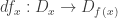
which behaves a lot like the differential of a smooth function. For example, the chain rule holds

$d(f\circ g)_x = df_{g(x)}\circ dg_x$

and if f is an equivalence, all induced $df_x$ are also equivalences. The latter corresponds to the fact that the differential of a diffeomorphism is invertible.
If we have a 0-group G with unit e, the left tranlations $g\cdot\_:\equiv x\mapsto g\cdot x$ are a family of equivalences that consistently identify $D_e$ with all other formal disks $D_x$ in G given by the differentials $d(g\cdot\_)_e$ .
This is essentially a generalization of the fact, that the tangent bundle of a Lie-group is trivialized by left translations and a solution to the first part of the first of Urs Schreiber’s problems I mentioned in the beginning.

With the exception of the chain rule, all of this was in my dissertation, which I defended in 2017. A couple of month ago, I wrote an article about this and put it on the arxiv and since monday, there is an improved version with an introduction that explains what monads $\Im$ you can think of and relates the setup to Synthetic Differential Geometry.
There is also a recording on youtube of a talk I gave about this in Bonn.

HoTT 2019

Save the date! Next summer will be the first:

International Conference on Homotopy Type Theory
(HoTT 2019)
Carnegie Mellon University
12 – 17 August 2019

There will also be an associated:

HoTT Summer School
7 – 10 August 2019

More details to follow soon!

Here is the conference website.

UF-IAS-2012 wiki archived

The wiki used for the 2012-2013 Univalent Foundations program at the Institute for Advanced Study was hosted at a provider called Wikispaces. After the program was over, the wiki was no longer used, but was kept around for historical and archival purposes; much of it is out of date, but it still contains some content that hasn’t been reproduced anywhere else.

Unfortunately, Wikispaces is closing, so the UF-IAS-2012 wiki will no longer be accessible there. With the help of Richard Williamson, we have migrated all of its content to a new archival copy hosted on the nLab server:

Archival copy of UF program wiki.

Let us know if you find any formatting or other problems.

A self-contained, brief and complete formulation of Voevodsky’s univalence axiom

I have often seen competent mathematicians and logicians, outside our circle, making technically erroneous comments about the univalence axiom, in conversations, in talks, and even in public material, in journals or the web.

For some time I was a bit upset about this. But maybe this is our fault, by often trying to explain univalence only imprecisely, mixing the explanation of the models with the explanation of the underlying Martin-Löf type theory, with none of the two explained sufficiently precisely.

There are long, precise explanations such as the HoTT book, for example, or the various formalizations in Coq, Agda and Lean.

But perhaps we don’t have publicly available material with a self-contained, brief and complete formulation of univalence, so that interested mathematicians and logicians can try to contemplate the axiom in a fully defined form.

So here is an attempt of a self-contained, brief and complete formulation of Voevodsky’s Univalence Axiom in the arxiv.

This has an Agda file with univalence defined from scratch as an ancillary file, without the use of any library at all, to try to show what the length of a self-contained definition of the univalence type is. Perhaps somebody should add a Coq “version from scratch” of this.

There is also a web version UnivalenceFromScratch to try to make this as accessible as possible, with the text and the Agda code together.

The above notes explain the univalence axiom only. Regarding its role, we recommend Dan Grayson’s introduction to univalent foundations for mathematicians.

HoTT at JMM

At the 2018 U.S. Joint Mathematics Meetings in San Diego, there will be an AMS special session about homotopy type theory. It’s a continuation of the HoTT MRC that took place this summer, organized by some of the participants to especially showcase the work done during and after the MRC workshop. Following is the announcement from the organizers.

We are pleased to announce the AMS Special Session on Homotopy Type Theory, to be held on January 11, 2018 in San Diego, California, as part of the Joint Mathematics Meetings (to be held January 10 – 13).

Homotopy Type Theory (HoTT) is a new field of study that relates constructive type theory to abstract homotopy theory. Types are regarded as synthetic spaces of arbitrary dimension and type equality as homotopy equivalence. Experience has shown that HoTT is able to represent many mathematical objects of independent interest in a direct and natural way. Its foundations in constructive type theory permit the statement and proof of theorems about these objects within HoTT itself, enabling formalization in proof assistants and providing a constructive foundation for other branches of mathematics.

This Special Session is affiliated with the AMS Mathematics Research Communities (MRC) workshop for early-career researchers in Homotopy Type Theory organized by Dan Christensen, Chris Kapulkin, Dan Licata, Emily Riehl and Mike Shulman, which took place last June.

The Special Session will include talks by MRC participants, as well as by senior researchers in the field, on various aspects of higher-dimensional type theory including categorical semantics, computation, and the formalization of mathematical theories. There will also be a panel discussion featuring distinguished experts from the field.

Further information about the Special Session, including a schedule and abstracts, can be found at: http://jointmathematicsmeetings.org/meetings/national/jmm2018/2197_program_ss14.html.
Please note that the early registration deadline is December 20, 2017.

If you have any questions about about the Special Session, please feel free to contact one of the organizers. We look forward to seeing you in San Diego.

Simon Cho (University of Michigan)
Liron Cohen (Cornell University)
Ed Morehouse (Wesleyan University)

Impredicative Encodings of Inductive Types in HoTT

I recently completed my master’s thesis under the supervision of Steve Awodey and Jonas Frey. A copy can be found here.

Known impredicative encodings of various inductive types in System F, such as the type

$\forall X. (X\rightarrow X) \rightarrow X \rightarrow X,$

of natural numbers do not satisfy the relevant $\eta$ -computation rules. The aim of this work is to refine the System F encodings by moving to a system of HoTT with an impredicative universe, so that the relevant $\eta$ -rules are satisfied (along with all the other rules). As a result, the so-determined types have their expected universal properties. The main result is the construction of a type of natural numbers which is the initial algebra for the expected endofunctor $X\mapsto X+\mathbf{1}$ .

For the inductive types treated in the thesis, we do not use the full power of HoTT; we need only postulate $\Sigma$ -types, identity types, “large” $\Pi$ -types over an impredicative universe $\mathcal{U}$ and function extensionality. Having large $\Pi$ -types over an impredicative universe $\mathcal{U}$ means that given a type $\Gamma\vdash A \:\mathsf{type}$ and a type family $\Gamma, x:A \vdash B:\mathcal{U}$ , we may form the dependent function type

$\displaystyle{ \Gamma\vdash \prod_{x:A} B:\mathcal{U}}.$

Note that this type is in $\mathcal{U}$ even if $A$ is not.

We obtain a translation of System F types into type theory by replacing second order quantification by dependent products over $\mathcal U$ (or alternatively over the subtype of $\mathcal{U}$ given by some h-level).

For brevity, we will focus on the construction of the natural numbers (though in the thesis, the coproduct of sets and the unit type is first treated with special cases of this method). We consider categories of algebras for endofunctors:

$T:\mathbf{Set}\rightarrow\mathbf{Set},$

where the type of objects of $\mathbf{Set}$ is given by

$\mathsf{Set} :\equiv \displaystyle{\sum_{X:\mathcal{U}}}\mathsf{isSet}(X),$

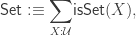
(the type of sets (in $\mathcal{U}$ )) and morphisms are simply functions between sets.

We can write down the type of $T$ -algebras:

$\mathsf{TAlg} :\equiv \displaystyle{\sum_{X:\mathsf{Set}}} T(X)\rightarrow X$

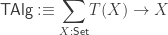
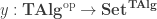
and homomorphisms between algebras $\phi$ and $\psi$ :

$\mathsf{THom}(\phi,\psi) :\equiv \displaystyle{\sum_{f:\mathsf{pr_1}(\phi)\rightarrow\mathsf{pr_1}(\psi)}} \mathsf{pr_2}(\psi) \circ T(f) = f \circ \mathsf{pr_2}(\phi),$

which together form the category $\mathbf{TAlg}$ .

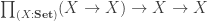
We seek the initial object in $\mathbf{TAlg}$ . Denote this by $0$ and moreover let $U$ be the forgetful functor to $\mathbf{Set}$ and $y:\mathbf{TAlg}^{\textnormal{op}}\rightarrow \mathbf{Set}^{\mathbf{TAlg}}$ be the covariant Yoneda embedding. We reason as follows:

$U0 \cong \textnormal{Hom}_{\mathbf{Set}^\mathbf{TAlg}}(y0,U) \\{}\:\,\,\,\,\,\, = \textnormal{Hom}_{\mathbf{Set}^\mathbf{TAlg}}(1,U) \\{}\:\,\,\,\,\,\, = \textnormal{Hom}_{\mathbf{Set}^\mathbf{TAlg}}(\Delta 1,U) \\{}\:\,\,\,\,\,\, = \textnormal{Hom}_{\mathbf{Set}}(1, \textnormal{lim}_{\phi\in\textbf{TAlg}} U\phi) \\{}\:\,\,\,\,\,\, \cong \textnormal{lim}_{\phi\in\textbf{TAlg}} U\phi,$

using the fact that the diagonal functor is left adjoint to the limit functor for the last step. With this, we have a proposal for the definition of the underlying set of the initial $T$ -algebra as the limit of the forgetful functor. Using the fact that $U0$ is defined as a limit, we obtain an algebra structure $\epsilon:TU0\rightarrow U0$ . As $U$ creates limits, $(U0,\epsilon)$ is guaranteed to be initial in $\mathbf{TAlg}$ .

But we want to define $U0$ in type theory. We do this using products and equalizers as is well known from category theory. Explicitly, we take the equalizer of the following two maps between products:

$P_1,P_2 : \left(\displaystyle{\prod_{\phi:\mathbf{TAlg}}}U(\phi)\right) \rightarrow \displaystyle{\prod_{\phi,\psi:\mathbf{TAlg}}} \: \displaystyle{\prod_{\mu:\mathbf{THom}(\phi,\psi)}}U(\psi),$

given by:

$P_1 :\equiv \lambda\Phi.\lambda\phi.\lambda\psi.\lambda\mu.\Phi(\psi), \\ P_1 :\equiv \lambda\Phi.\lambda\phi.\lambda\psi.\lambda\mu. \mathsf{pr_1}(\mu)(\Phi(\phi)).$

The equalizer is, of course:

$E :\equiv \displaystyle{\sum_{\Phi : \prod_{(\phi:\mathbf{TAlg})} U(\phi)}} P_1(\Phi)=P_2(\Phi),$

which inhabits $\mathsf{Set}$ . Impredicativity is crucial for this: it guarantees that the product over $\mathbf{TAlg}$ lands in $\mathcal{U}$ .

This method can be used to construct an initial algebra, and therefore a fixed-point, for any endofunctor $T : \mathsf{Set}\rightarrow\mathsf{Set}\,$ ! We won’t pursue this remarkable fact here, but only consider the case at hand, where the functor $T$ is $X\mapsto X+\mathbf{1}$ . Then the equalizer $E$ becomes our definition of the type of natural numbers (so let us rename $E$ to $\mathbb{N}$ for the remainder). Observe that this encoding can be seen as a subtype of (a translation of) the System F encoding given at the start. Indeed, the indexing object $\prod_{(\phi:\mathbf{TAlg})} U(\phi)$ of $E$ is equivalent to $\prod_{(X:\mathbf{Set})}(X\rightarrow X)\rightarrow X \rightarrow X$ , by

$\begin{aligned} \quad\quad\displaystyle{\prod_{\phi:\mathbf{TAlg}}} U(\phi) \quad &\cong\quad \displaystyle{\prod_{\phi:{\displaystyle{\sum_{X:\mathsf{Set}}} T(X)\rightarrow X}}} U(\phi)\\ &\cong\quad \displaystyle{\prod_{X:\mathsf{Set}}}\, \displaystyle{\prod_{f:T(X)\rightarrow X}} X\\ &\cong\quad \displaystyle{\prod_{X:\mathsf{Set}}}\, (T(X)\rightarrow X) \rightarrow X\\ &\cong\quad \displaystyle{\prod_{X:\mathbf{Set}}}(X\rightarrow X)\rightarrow X \rightarrow X \,. \end{aligned}$

With this, we can define a successor function and zero element, for instance:

$0 :\equiv \left( \lambda\phi. \mathsf{pr_2}(\phi)\mathsf{inr}(\star), \lambda\phi.\lambda\psi.\lambda\mu. \mathsf{refl}_{\mathsf{pr_2}(\psi)\mathsf{inr}(\star)}\right)$

(the successor function takes a little more work). We can also define a recursor $\mathsf{rec}_{\mathbb{N}}(e,c)$ , given any $C:\mathsf{Set}, e:C\rightarrow C$ and $c:C$ . In other words, the introduction rules hold, and we can eliminate into other sets. Further, the $\beta$ -rules hold definitionally – as expected, since they hold for the System F encodings.

Finally we come to the desired result, the $\eta$ -rule for $\mathbb{N}$ :

Theorem. Let $C:\mathsf{Set}, e:C\rightarrow C$ and $c:C$ . Moreover, let $f:\mathbb{N}\rightarrow C$ such that:

$f(0)=c, \\ f(\mathsf{succ}(x) = e(f(x))$

for any $x:\mathbb{N}$ . Then

$\mathsf{rec}_{\mathbb{N}}(e,c) =f.$

Note that the $\eta$ -rule holds propositionally. By Awodey, Gambino, and Sojakova we therefore also have, equivalently, the induction principle for $\mathbb{N}$ , aka the dependent elimination rule. As a corollary, we can prove the universal property that any $T$ -algebra homomorphism is propositionally equal to the appropriate recursor (as a $T$ -algebra homomorphism). Again we emphasise the need for impredicativity: in the proof of $\eta$ , we have to be able to plug $\mathbb{N}$ into quantifiers over $\mathsf{Set}$ .

A semantic rendering of the above is that we have built a type that always determines a natural numbers object—whereas the System F encoding need not always do so (see Rummelhoff). In an appendix, we discuss a realizability semantics for the system we work in. Building more exotic types (that need not be sets) becomes more complicated; we leave this to future work.

In memoriam: Vladimir Voevodsky

https://www.ias.edu/news/2017/vladimir-voevodsky

A hands-on introduction to cubicaltt

Some months ago I gave a series of hands-on lectures on cubicaltt at Inria Sophia Antipolis that can be found at:

https://github.com/mortberg/cubicaltt/tree/master/lectures

The lectures cover the main features of the system and don’t assume any prior knowledge of Homotopy Type Theory or Univalent Foundations. Only basic familiarity with type theory and proof assistants based on type theory is assumed. The lectures are in the form of cubicaltt files and can be loaded in the cubicaltt proof assistant.

cubicaltt is based on a novel type theory called Cubical Type Theory that provides new ways to reason about equality. Most notably it makes various extensionality principles, like function extensionality and Voevodsky’s univalence axiom, into theorems instead of axioms. This is done such that these principles have computational content and in particular that we can transport structures between equivalent types and that these transports compute. This is different from when one postulates the univalence axiom in a proof assistant like Coq or Agda. If one just adds an axiom there is no way for Coq or Agda to know how it should compute and one looses the good computational properties of type theory. In particular canonicity no longer holds and one can produce terms that are stuck (e.g. booleans that are neither true nor false but don’t reduce further). In other words this is like having a programming language in which one doesn’t know how to run the programs. So cubicaltt provides an operational semantics for Homotopy Type Theory and Univalent Foundations by giving a computational justification for the univalence axiom and (some) higher inductive types.

Cubical Type Theory has a model in cubical sets with lots of structure (symmetries, connections, diagonals) and is hence consistent. Furthermore, Simon Huber has proved that Cubical Type Theory satisfies canonicity for natural numbers which gives a syntactic proof of consistency. Many of the features of the type theory are very inspired by the model, but for more syntactically minded people I believe that it is definitely possible to use cubicaltt without knowing anything about the model. The lecture notes are hence written with almost no references to the model.

The cubicaltt system is based on Mini-TT:

"A simple type-theoretic language: Mini-TT" (2009)
Thierry Coquand, Yoshiki Kinoshita, Bengt Nordström and Makoto Takeya
In "From Semantics to Computer Science; Essays in Honour of Gilles Kahn"

Mini-TT is a variant Martin-Löf type theory with datatypes and cubicaltt extends Mini-TT with:

Path types
Compositions
Glue types
Id types
Some higher inductive types

The lectures cover the first 3 of these and hence correspond to sections 2-7 of:

"Cubical Type Theory: a constructive interpretation of the univalence axiom"
Cyril Cohen, Thierry Coquand, Simon Huber and Anders Mörtberg
To appear in post-proceedings of TYPES 2016
https://arxiv.org/abs/1611.02108

I should say that cubicaltt is mainly meant to be a prototype implementation of Cubical Type Theory in which we can do experiments, however it was never our goal to implement a competitor to any of the more established proof assistants. Because of this there are no implicit arguments, type classes, proper universe management, termination checker, etc… Proofs in cubicaltt hence tend to get quite verbose, but it is definitely possible to do some fun things. See for example:

binnat.ctt – Binary natural numbers and isomorphism to unary numbers. Example of data and program refinement by doing a proof for unary numbers by computation with binary numbers.
setquot.ctt – Formalization of impredicative set quotients á la Voevodsky.
hz.ctt – $\mathbb{Z}$ defined as an (impredicative set) quotient of nat * nat.
category.ctt – Categories. Structure identity principle. Pullbacks. (Due to Rafaël Bocquet)
csystem.ctt – Definition of C-systems and universe categories. Construction of a C-system from a universe category. (Due to Rafaël Bocquet)

For a complete list of all the examples see:

https://github.com/mortberg/cubicaltt/tree/master/examples

For those who cannot live without implicit arguments and other features of modern proof assistants there is now an experimental cubical mode shipped with the master branch of Agda. For installation instructions and examples see:

https://agda.readthedocs.io/en/latest/language/cubical.html
https://github.com/Saizan/cubical-demo

In this post I will give some examples of the main features of cubicaltt, but for a more comprehensive introduction see the lecture notes. As cubicaltt is an experimental prototype things can (and probably will) change in the future (e.g. see the paragraph on HITs below).

The basic type theory

The basic type theory on which cubicaltt is based has Π and ∑ types (with eta and surjective pairing), a universe U, datatypes, recursive definitions and mutually recursive definitions (in particular inductive-recursive definitions). Note that general datatypes and (mutually recursive) definitions are not part of the version of Cubical Type Theory in the paper.

Below is an example of how natural numbers and addition are defined:

data nat = zero

| suc (n : nat)

add (m : nat) : nat -> nat = split

zero -> m

suc n -> suc (add m n)

If one loads this in the cubicaltt read-eval-print-loop one can compute things:

> add (suc zero) (suc zero)

EVAL: suc (suc zero)

Path types

The homotopical interpretation of equality tells us that we can think of an equality proof between a and b in a type A as a path between a and b in a space A. cubicaltt takes this literally and adds a primitive Path type that should be thought of as a function out of an abstract interval $\mathbb{I}$ with fixed endpoints.

We call the elements of the interval $\mathbb{I}$ names/directions/dimensions and typically use i, j, k to denote them. The elements of the interval $\mathbb{I}$ are generated by the following grammar (where dim is a dimension like i, j, k…):

r,s := 0
     | 1
     | dim
     | - r
     | r /\ s
     | r \/ s

The endpoints are 0 and 1, – corresponds to symmetry (r in $\mathbb{I}$ is mapped to 1-r), while /\ and \/ are so called “connections”. The connections can be thought of mapping r and s in $\mathbb{I}$ to min(r,s) and max(r,s) respectively. As Path types behave like functions out of the interval there is both path abstraction and application (just like for function types). Reflexivity is written:

refl (A : U) (a : A) : Path A a a = a

and corresponds to a constant path:

        <i> a
   a -----------> a

with the intuition is that  a is a function \(i : ) -> a. However for deep reasons the interval isn’t a type (as it isn’t fibrant) so we cannot write functions out of it directly and hence we have this special notation for path abstraction.

If we have a path from a to b then we can compute its left end-point by applying it to 0:

face0 (A : U) (a b : A) (p : Path A a b) : A = p @ 0

This is of course convertible to a. We can also reverse a path by using symmetry:

sym (A : U) (a b : A) (p : Path A a b) : Path A b a =

 p @ -i

Assuming that some arguments could be made implicit this satisfies the equality

sym (sym p) == p

judgmentally. This is one of many examples of equalities that hold judgmentally in cubicaltt but not in standard type theory where sym would be defined by induction on p. This is useful for formalizing mathematics, for example we get the judgmental equality C^op^op == C for a category C that cannot be obtained in standard type theory with the usual definition of category without using any tricks (see opposite.ctt for a formal proof of this).

We can also directly define cong (or ap or mapOnPath):

cong (A B : U) (f : A -> B) (a b : A) (p : Path A a b) :

Path B (f a) (f b) = f (p @ i)

Once again this satisfies some equations judgmentally that we don’t get in standard type theory where this would have been defined by induction on p:

cong id p == p

cong g (cong f p) == cong (g o f) p

Finally the connections can be used to construct higher dimensional cubes from lower dimensional ones (e.g. squares from lines). If p : Path A a b then  p @ i /\ j is the interior of the square:

                  p
        a -----------------> b
        ^                    ^
        |                    |
        |                    |
  <j> a |                    | p
        |                    |
        |                    |
        |                    |
        a -----------------> a
                <i> a

Here i corresponds to the left-to-right dimension and j corresponds to the down-to-up dimension. To compute the left and right sides just plug in i=0 and i=1 in the term inside the square:

<j> p @ 0 /\ j = <j> p @ 0 = <j> a   (p is a path from a to b)
<j> p @ 1 /\ j = <j> p @ j = p       (using eta for Path types)

These give a short proof of contractibility of singletons (i.e. that the type (x : A) * Path A a x is contractible for all a : A), for details see the lecture notes or the paper. Because connections allow us to build higher dimensional cubes from lower dimensional ones they are extremely useful for reasoning about higher dimensional equality proofs.

Another cool thing with Path types is that they allow us to give a direct proof of function extensionality by just swapping the path and lambda abstractions:

funExt (A B : U) (f g : A -> B)

(p : (x : A) -> Path B (f x) (g x)) :

Path (A -> B) f g = \(a : A) -> (p a) @ i

To see that this makes sense we can compute the end-points:

(<i> \(a : A) -> (p a) @ i) @ 0 = \(a : A) -> (p a) @ 0
                                = \(a : A) -> f a
                                = f

and similarly for the right end-point. Note that the last equality follows from eta for Π types.

We have now seen that Path types allows us to define the constants of HoTT (like cong or funExt), but when doing proofs with Path types one rarely uses these constants explicitly. Instead one can directly prove things with the Path type primitives, for example the proof of function extensionality for dependent functions is exactly the same as the one for non-dependent functions above.

We cannot yet prove the principle of path induction (or J) with what we have seen so far. In order to do this we need to be able to turn any path between types A and B into a function from A to B, in other words we need to be able to define transport (or cast or coe):

transport : Path U A B -> A -> B

Composition, filling and transport

The computation rules for the transport operation in cubicaltt is introduced by recursion on the type one is transporting in. This is quite different from traditional type theory where the identity type is introduced as an inductive family with one constructor (refl). A difficulty with this approach is that in order to be able to define transport in a Path type we need to keep track of the end-points of the Path type we are transporting in. To solve this we introduce a more general operation called composition.

Composition can be used to define the composition of paths (hence the name). Given paths p : Path A a b and q : Path A b c the composite is obtained by computing the missing top line of this open square:

        a                   c
        ^                   ^
        |                   |
        |                   |
  <j> a |                   | q
        |                   |
        |                   |
        |                   |
        a ----------------> b
                p @ i

In the drawing I’m assuming that we have a direction i : in context that goes left-to-right and that the j goes down-to-up (but it’s not in context, rather it’s implicitly bound by the comp operation). As we are constructing a Path from a to c we can use the i and put p @ i as bottom. The code for this is as follows:

compPath (A : U) (a b c : A)

(p : Path A a b) (q : Path A b c) : Path A a c =

 comp (<_> A) (p @ i)

[ (i = 0) -> <j> a

, (i = 1) -> q ]

One way to summarize what compositions gives us is the so called “box principle” that says that “any open box has a lid”. Here “box” means (n+1)-dimensional cube and the lid is an n-dimensional cube. The comp operation takes as second argument the bottom of the box and then a list of sides. Note that the collection of sides doesn’t have to be exhaustive (as opposed to the original cubical set model) and one way to think about the sides is as a collection of constraints that the resulting lid has to satisfy. The first argument of comp is a path between types, in the above example this path is constant but it doesn’t have to be. This is what allows us to define transport:

transport (A B : U) (p : Path U A B) (a : A) : B =

comp p a []

Combining this with the contractibility of singletons we can easily prove the elimination principle for Path types. However the computation rule does not hold judgmentally. This is often not too much of a problem in practice as the Path types satisfy various judgmental equalities that normal Id types don’t. Also, having the possibility to reason about higher equalities directly using path types and compositions is often very convenient and leads to very nice and new ways to construct proofs about higher equalities in a geometric way by directly reasoning about higher dimensional cubes.

The composition operations are related to the filling operations (as in Kan simplicial sets) in the sense that the filling operations takes an open box and computes a filler with the composition as one of its faces. One of the great things about cubical sets with connections is that we can reduce the filling of an open box to its composition. This is a difference compared to the original cubical set model and it provides a significant simplification as we only have to explain how to do compositions in open boxes and not also how to fill them.

Glue types and univalence

The final main ingredient of cubicaltt are the Glue types. These are what allows us to have a direct algorithm for composition in the universe and to prove the univalence axiom. These types add the possibility to glue types along equivalences (i.e. maps with contractible fibers) onto another type. In particular this allows us to directly define one of the key ingredients of the univalence axiom:

ua (A B : U) (e : equiv A B) : Path U A B =

 Glue B [ (i = 0) -> (A,e)

, (i = 1) -> (B,idEquiv B) ]

This corresponds to the missing line at the top of:

        A           B
        |           |
      e |           | idEquiv B
        |           |
        V           V
        B --------> B
              B

The sides of this square are equivalences while the bottom and top are lines in direction i (so this produces a path from A to B as desired).

We have formalized three proofs of the univalence axiom in cubicaltt:

A very direct proof due to Simon Huber and me using higher dimensional glueing.
The more conceptual proof from section 7.2 of the paper in which we show that the unglue function is an equivalence (formalized by Fabian Ruch).
A proof from ua and its computation rule (uabeta). Both of these constants are easy to define and are sufficient for the full univalence axiom as noted in a post by Dan Licata on the HoTT google group.

All of these proofs can be found in the file univalence.ctt and are explained in the paper (proofs 1 and 3 are in Appendix B).

Note that one often doesn’t need full univalence to do interesting things. So just like for Path types it’s often easier to just use the Glue primitives directly instead of invoking the full univalence axiom. For instance if we have proved that negation is an involution for bool we can directly get a non-trivial path from bool to bool using ua (which is just a Glue):

notEq : Path U bool bool = ua boob bool notEquiv

And we can use this non-trivial equality to transport true and compute the result:

> transport notEq true

EVAL: false

This is all that the lectures cover, in the rest of this post I will discuss the two extensions of cubicaltt from the paper and their status in cubicaltt.

Identity types and higher inductive types

As pointed out above the computation rule for Path types doesn’t hold judgmentally. Luckily there is a neat trick due to Andrew Swan that allows us to define a new type that is equivalent to Path A a b for which the computation rule holds judgmentally. For details see section 9.1 of the paper. We call this type Id A a b as it corresponds to Martin-Löf’s identity type. We have implemented this in cubicaltt and proved the univalence axiom expressed exclusively using Id types, for details see idtypes.ctt.

For practical formalizations it is probably often more convenient to use the Path types directly as they have the nice primitives discussed above, but the fact that we can define Id types is very important from a theoretical point of view as it shows that cubicaltt with Id is really an extension of Martin-Löf type theory. Furthermore as we can prove univalence expressed using Id types we get that any proof in univalent type theory (MLTT extended with the univalence axiom) can be translated into cubicaltt.

The second extension to cubicaltt are HITs. We have a general syntax for adding these and some of them work fine on the master branch, see for example:

circle.ctt – The circle as a HIT. Computation of winding numbers.
helix.ctt – The loop space of the circle is equal to Z.
susp.ctt – Suspension and n-spheres.
torsor.ctt – Torsors. Proof that S1 is equal to BZ, the classifying
space of Z. (Due to Rafaël Bocquet)
torus.ctt – Proof that Torus = S1 * S1 in only 100 loc (due to Dan
Licata).

However there are various known issues with how the composition operations compute for recursive HITs (e.g. truncations) and HITs where the end-points contain function applications (e.g. pushouts). We have a very experimental branch that tries to resolve these issues called “hcomptrans”. This branch contains some new (currently undocumented) primitives that we are experimenting with and so far it seems like these are solving the various issues for the above two classes of more complicated HITs that don’t work on the master branch. So hopefully there will soon be a new cubical type theory with support for a large class of HITs.

That’s all I wanted to say about cubicaltt in this post. If someone plays around with the system and proves something cool don’t hesitate to file a pull request or file issues if you find some bugs.

Type theoretic replacement & the n-truncation

This post is to announce a new article that I recently uploaded to the arxiv:

https://arxiv.org/abs/1701.07538

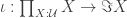
The main result of that article is a type theoretic replacement construction in a univalent universe that is closed under pushouts. Recall that in set theory, the replacement axiom asserts that if $F$ is a class function, assigning to any set $X$ a new set $F(X)$ , then the image of any set $A$ , i.e. the set $\{F(X)\mid X\in A\}$ is again a set. In homotopy type theory we consider instead a map $f : A\to X$ from a small type $A:U$ into a locally small type $X$ , and our main result is the construction of a small type $\mathrm{im}(f)$ with the universal property of the image of $f$ .

We say that a type is small if it is in $U$ , and for the purpose of this blog post smallness and locally smallness will always be with respect to $U$ . Before we define local smallness, let us recall the following rephrasing of the `encode-decode method’, which we might also call the Licata-Shulman theorem:

Theorem. Let $A$ be a type with $a:A$ , and let $P: A\to U$ be a type with $p:P(a)$ . Then the following are equivalent.

The total space $\Sigma_{(b:A)} P(b)$ is contractible.
The canonical map $\Pi_{(b:A)} (a=b)\to P(b)$ defined by path induction, mapping $\mathrm{refl}_a$ to $p$ , is a fiberwise equivalence.

Note that this theorem follows from the fact that a fiberwise map is a fiberwise equivalence if and only if it induces an equivalence on total spaces. Since for path spaces the total space will be contractible, we observe that any fiberwise equivalence establishes contractibility of the total space, i.e. we might add the following equivalent statement to the theorem.

There (merely) exists a family of equivalences $e:\Pi_{(b:B)} (a=b)\simeq P(b)$ . In other words, $P$ is in the connected component of the type family $b\mapsto (a=b)$ .

There are at least two equivalent ways of saying that a (possibly large) type $X$ is locally small:

For each $x,y:X$ there is a type $(x='y):U$ and an equivalence $e_{x,y}:(x=y)\simeq (x='y)$ .
For each $x,y:X$ there is a type $(x='y):U$ ; for each $x:X$ there is a term $r_X:x='x$ , and the canonical dependent function $\Pi_{(y:X)} (x=y)\to (x='y)$ defined by path induction by sending $\mathrm{refl}_x$ to $r_x$ is an equivalence.

Note that the data in the first structure is clearly a (large) mere proposition, because there can be at most one such a type family $(x='y)$ , while the equivalences in the second structure are canonical with respect to the choice of reflexivity $r_x$ . To see that these are indeed equivalent, note that the family of equivalences in the first structure is a fiberwise equivalence, hence it induces an equivalence on total spaces. Therefore it follows that the total space $\Sigma_{(y:X)} (x='y)$ is contractible. Thus we see by Licata’s theorem that the canoncial fiberwise map is a fiberwise equivalence. Furthermore, it is not hard to see that the family of equivalences $e_{x,y}$ is equal to the canonical family of equivalences. There is slightly more to show, but let us keep up the pace and go on.

Examples of locally small types include any small type, any mere proposition regardless of their size, the universe is locally small by the univalence axiom, and if $A$ is small and $X$ is locally small then the type $A\to X$ is locally small. Observe also that the univalence axiom follows if we assume the `uncanonical univalence axiom’, namely that there merely exists a family of equivalences $e_{A,B} : (A=B)\simeq (A\simeq B)$ . Thus we see that the slogan ‘identity of the universe is equivalent to equivalence’ actually implies univalence.

Main Theorem. Let $U$ be a univalent universe that is closed under pushouts. Suppose that $A:U$ , that $X$ is a locally small type, and let $f:A\to X$ . Then we can construct

a small type $\mathrm{im}(f):U$ ,
a factorization
such that $i_f$ is an embedding that satisfies the universal property of the image inclusion, namely that for any embedding $g$ , of which the domain is possibly large, if $f$ factors through $g$ , then so does $i_f$ .

Recall that $f$ factors through an embedding $g$ in at most one way. Writing $\mathrm{Hom}_X(f,g)$ for the mere proposition that $f$ factors through $g$ , we see that $i_f$ satisfies the universal property of the image inclusion precisely when the canonical map

$\mathrm{Hom}_X(i_f,g)\to\mathrm{Hom}_X(f,g)$

is an equivalence.

Most of the paper is concerned with the construction with which we prove this theorem: the join construction. By repeatedly joining a map with itself, one eventually arrives at an embedding. The join of two maps $f:A\to X$ and $g:B\to X$ is defined by first pulling back, and then taking the pushout, as indicated in the following diagram

In the case $X \equiv \mathbf{1}$ , the type $A \ast_X B$ is equivalent to the usual join of types $A \ast B$ . Just like the join of types, the join of maps with a common codomain is associative, commutative, and it has a unit: the unique map from the empty type into $X$ . The join of two embeddings is again an embedding. We show that the last statement can be strengthened: the maps $f:A\to X$ that are idempotent in a canonical way (i.e. the canonical morphism $f \to f \ast f$ in the slice category over $X$ is an equivalence) are precisely the embeddings.

Below, I will indicate how we can use the above theorem to construct the n-truncations for any $n\geq -2$ on any univalent universe that is closed under pushouts. Other applications include the construction of set-quotients and of Rezk-completion, since these are both constructed as the image of the Yoneda-embedding, and it also follows that the univalent completion of any dependent type $P:A\to U$ can be constructed as a type in $U$ , namely $\mathrm{im}(P)$ , without needing to resort to more exotic higher inductive types. In particular, any connected component of the universe is equivalent to a small type.

Theorem. Let $U$ be a univalent universe that is closed under pushouts. Then we can define for any $n\geq -2$

an n-truncation operation $\|{-}\|_n:U\to U$ ,
a map $|{-}|:\Pi_{(A:U)} A\to \|A\|_n$
such that for any $A:U$ , the type $\|A\|_n$ is n-truncated and satisfies the (dependent) universal property of n-truncation, namely that for every type family $P:\|A\|_n\to\mathrm{Type}$ of possibly large types such that each $P(x)$ is n-truncated, the canonical map
$(\Pi_{(x:\|A\|_n)} P(x))\to (\Pi_{(a:A)} P(|a|_n))$
given by precomposition by $|{-}|_n$ is an equivalence.

Construction. The proof is by induction on $n\geq -2$ . The case $n\equiv -2$ is trivial (take $A\mapsto \mathbf{1}$ ). For the induction hypothesis we assume an n-truncation operation with structure described in the statement of the theorem.

First, we define $\mathcal{Y}_n:A\to (A\to U)$ by $\mathcal{Y}_n(a,b):\equiv \|a=b\|_n$ . As we have seen, the universe is locally small, and therefore the type $A\to U$ is locally small. Therefore we can define

$\|A\|_{n+1} :\equiv \mathrm{im}(\mathcal{Y}_n)$
$|{-}|_{n+1} :\equiv q_{\mathcal{Y}_n}$ .

For the proof that $\|A\|_{n+1}$ is indeed $(n+1)$ -truncated, and satisfies the universal property of the n-truncation we refer to the article.

Parametricity, automorphisms of the universe, and excluded middle

Specific violations of parametricity, or existence of non-identity automorphisms of the universe, can be used to prove classical axioms. The former was previously featured on this blog, and the latter is part of a discussion on the HoTT mailing list. In a cooperation between Martín Escardó, Peter Lumsdaine, Mike Shulman, and myself, we have strengthened these results and recorded them in a paper that is now on arXiv.

In this blog post, we work with the full repertoire of HoTT axioms, including univalence, propositional truncations, and pushouts. For the paper, we have carefully analysed which assumptions are used in which theorem, if any.

Parametricity

Parametricity is a property of terms of a language. If your language only has parametric terms, then polymorphic functions have to be invariant under the type parameter. So in MLTT, the only term inhabiting the type $\prod_{X:\mathcal{U}}X \to X$ of polymorphic endomaps is the polymorphic identity $\lambda (X:\mathcal{U}). \mathsf{id}_X$ .

In univalent foundations, we cannot prove internally that every term is parametric. This is because excluded middle is not parametric (exercise 6.9 of the HoTT book tells us that, assuming LEM, we can define a polymorphic endomap that flips the booleans), but there exist classical models of univalent foundations. So if we could prove this internally, excluded middle would be false, and thus the classical models would be invalid.

In the abovementioned blog post, we observed that exercise 6.9 of the HoTT book has a converse: if $f:\prod_{X:\mathcal{U}}X\to X$ is the flip map on the type of booleans, then excluded middle holds. In the paper on arXiv, we have a stronger result:

Theorem. There exist $f:\prod_{X:\mathcal{U}}X\to X$ and a type $X$ and a point $x:X$ with $f_X(x)\neq x$ if and only if excluded middle holds.

Notice that there are no requirements on the type $X$ or the point $x$ . We have also applied the technique used for this theorem in other scenarios, for example:

Theorem. There exist $f:\prod_{X:\mathcal{U}}X\to \mathbf{2}$ and types $X, Y$ and points $x:X, y:Y$ with $f_X(x)\neq f_Y(y)$ if and only if weak excluded middle holds.

The results in the paper illustrate that different violations of parametricity have different proof-theoretic strength: some violations are impossible, while others imply varying amounts of excluded middle.

Automorphisms of the universe

In contrast to parametricity, which proves that terms of some language necessarily have some properties, it is currently unknown if non-identity automorphisms of the universe are definable in univalent foundations. But some believe that this may not be the case.

In the presence of excluded middle, we can define non-identity automorphisms of the universe. Given a type $X$ , we use excluded middle to decide if $X$ is a proposition. If it is, we map $X$ to $\neg X$ , and otherwise we map $X$ to itself. Assuming excluded middle, we have $\neg\neg X=X$ for any proposition, so this is an automorphism.

The above automorphism swaps the empty type $\mathbf{0}$ with the unit type $\mathbf{1}$ and leaves all other types unchanged. More generally, assuming excluded middle we can swap any two types with equivalent automorphism ∞-groups, since in that case the corresponding connected components of the universe are equivalent. Still more generally, we can permute arbitrarily any family of types all having the same automorphism ∞-group.

The simplest case of this is when all the types are rigid, i.e. have trivial automorphism ∞-group. The types $\mathbf{0}$ and $\mathbf{1}$ are both rigid, and at least with excluded middle no other sets are; but there can be rigid higher types. For instance, if $G$ is a group that is a set (i.e. a 1-group), then its Eilenberg-Mac Lane space $B G$ is a 1-type, and its automorphism ∞-group is a 1-type whose $\pi_0$ is the outer automorphisms of $G$ and whose $\pi_1$ is the center of $G$ . Thus, if $G$ has trivial outer automorphism group and trivial center, then $BG$ is rigid. Such groups are not uncommon, including for instance the symmetric group $S_n$ for any $n\neq 2,6$ . Thus, assuming excluded middle we can permute these $BS_n$ arbitrarily, producing uncountably many automorphisms of the universe.

In the converse direction, we recorded the following.

Theorem. If there is an automorphism of the universe that maps some inhabited type to the empty type, then excluded middle holds.

Corollary. If there is an automorphism $g:\mathcal{U}\to\mathcal{U}$ of the universe with $g(\mathbf{0})\neq\mathbf{0}$ , then the double negation

$\neg\neg\prod_{P:\mathcal{U}}\mathsf{isProp}(P)\to P+\neg P$

of the law of excluded middle holds.

This corollary relates to an unclaimed prize: if from an arbitrary equivalence $f:\mathcal{U}\to\mathcal{U}$ such that $f(X) \neq X$ for a particular $X:\mathcal{U}$ you get a non-provable consequence of excluded middle, then you get $X$ -many beers. So this corollary wins you 0 beers. Although perhaps sober, we think this is an achievement worth recording.

Using this corollary, in turn, we can win $\mathsf{LEM}_\mathcal{U}$ -many beers, where $\mathsf{LEM}_\mathcal{U}$ is excluded middle for propositions in the universe $\mathcal{U}$ . If $\mathcal{U} :\mathcal{V}$ we have $\mathsf{LEM}_\mathcal{U}:\mathcal{V}$ . Suppose $g$ is an automorphism of $\mathcal{V}$ with $g(\mathsf{LEM}_\mathcal{U})\neq\mathsf{LEM}_\mathcal{U}$ , then $\neg\neg\mathsf{LEM}_\mathcal{U}$ . For suppose that $\neg\mathsf{LEM}_\mathcal{U}$ , and hence $\mathsf{LEM}_\mathcal{U}=\mathbf{0}$ . So by the corollary, we obtain $\neg\neg\mathsf{LEM}_\mathcal{V}$ . But $\mathsf{LEM}_\mathcal{V}$ implies $\mathsf{LEM}_\mathcal{U}$ by cumulativity, so $\neg\neg\mathsf{LEM}_\mathcal{U}$ also holds, contradicting our assumption that $\neg\mathsf{LEM}_\mathcal{U}$ .

To date no one has been able to win 1 beer.

HoTTSQL: Proving Query Rewrites with Univalent SQL Semantics

SQL is the lingua franca for retrieving structured data. Existing semantics for SQL, however, either do not model crucial features of the language (e.g., relational algebra lacks bag semantics, correlated subqueries, and aggregation), or make it hard to formally reason about SQL query rewrites (e.g., the SQL standard’s English is too informal). This post focuses on the ways that HoTT concepts (e.g., Homotopy Types, the Univalence Axiom, and Truncation) enabled us to develop HoTTSQL — a new SQL semantics that makes it easy to formally reason about SQL query rewrites. Our paper also details the rich set of SQL features supported by HoTTSQL.

You can download this blog post’s source (implemented in Coq using the HoTT library). Learn more about HoTTSQL by visiting our website.

Continue reading →

Combinatorial Species and Finite Sets in HoTT

(Post by Brent Yorgey)

My dissertation was on the topic of combinatorial species, and specifically on the idea of using species as a foundation for thinking about generalized notions of algebraic data types. (Species are sort of dual to containers; I think both have intereseting and complementary things to offer in this space.) I didn’t really end up getting very far into practicalities, instead getting sucked into a bunch of more foundational issues.

To use species as a basis for computational things, I wanted to first “port” the definition from traditional, set-theory-based, classical mathematics into a constructive type theory. HoTT came along at just the right time, and seems to provide exactly the right framework for thinking about a constructive encoding of combinatorial species.

For those who are familiar with HoTT, this post will contain nothing all that new. But I hope it can serve as a nice example of an “application” of HoTT. (At least, it’s more applied than research in HoTT itself.)

Combinatorial Species

Traditionally, a species is defined as a functor 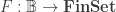$F : \mathbb{B} \to \mathbf{FinSet}$ , where $\mathbb{B}$ is the groupoid of finite sets and bijections, and $\mathbf{FinSet}$ is the category of finite sets and (total) functions. Intuitively, we can think of a species as mapping finite sets of “labels” to finite sets of “structures” built from those labels. For example, the species of linear orderings (i.e. lists) maps the finite set of labels $\{1,2, \dots, n\}$ to the size- $n!$ set of all possible linear orderings of those labels. Functoriality ensures that the specific identity of the labels does not matter—we can always coherently relabel things.

Constructive Finiteness

So what happens when we try to define species inside a constructive type theory? The crucial piece is $\mathbb{B}$ : the thing that makes species interesting is that they have built into them a notion of bijective relabelling, and this is encoded by the groupoid $\mathbb{B}$ . The first problem we run into is how to encode the notion of a finite set, since the notion of finiteness is nontrivial in a constructive setting.

One might well ask why we even care about finiteness in the first place. Why not just use the groupoid of all sets and bijections? To be honest, I have asked myself this question many times, and I still don’t feel as though I have an entirely satisfactory answer. But what it seems to come down to is the fact that species can be seen as a categorification of generating functions. Generating functions over the semiring $R$ can be represented by functions $\mathbb{N} \to R$ , that is, each natural number maps to some coefficient in $R$ ; each natural number, categorified, corresponds to (an equivalence class of) finite sets. Finite label sets are also important insofar as our goal is to actually use species as a basis for computation. In a computational setting, one often wants to be able to do things like enumerate all labels (e.g. in order to iterate through them, to do something like a map or fold). It will therefore be important that our encoding of finiteness actually has some computational content that we can use to enumerate labels.

Our first attempt might be to say that a finite set will be encoded as a type $A$ together with a bijection between $A$ and a canonical finite set of a particular natural number size. That is, assuming standard inductively defined types $\mathbb{N}$ and $\mathsf{Fin}$ ,

$\displaystyle \Sigma (A:U). \Sigma (n : \mathbb{N}). A \cong \mathsf{Fin}(n).$

However, this is unsatisfactory, since defining a suitable notion of bijections/isomorphisms between such finite sets is tricky. Since $\mathbb{B}$ is supposed to be a groupoid, we are naturally led to try using equalities (i.e. paths) as morphisms—but this does not work with the above definition of finite sets. In $\mathbb{B}$ , there are supposed to be $n!$ different morphisms between any two sets of size $n$ . However, given any two same-size inhabitants of the above type, there is only one path between them—intuitively, this is because paths between $\Sigma$ -types correspond to tuples of paths relating the components pointwise, and such paths must therefore preserve the particular relation to $\mathsf{Fin}(n)$ . The only bijection which is allowed is the one which sends each element related to $i$ to the other element related to $i$ , for each $i \in \mathsf{Fin}(n)$ .

So elements of the above type are not just finite sets, they are finite sets with a total order, and paths between them must be order-preserving; this is too restrictive. (However, this type is not without interest, and can be used to build a counterpart to L-species. In fact, I think this is exactly the right setting in which to understand the relationship between species and L-species, and more generally the difference between isomorphism and equipotence of species; there is more on this in my dissertation.)

Truncation to the Rescue

We can fix things using propositional truncation. In particular, we define

$\displaystyle U_F := \Sigma (A:U). \|\Sigma (n : \mathbb{N}). A \cong \mathsf{Fin}(n)\|.$

That is, a “finite set” is a type $A$ together with some hidden evidence that $A$ is equivalent to $\mathsf{Fin}(n)$ for some $n$ . (I will sometimes abuse notation and write $A : U_F$ instead of $(A, p) : U_F$ .) A few observations:

First, we can pull the size $n$ out of the propositional truncation, that is, $U_F \cong \Sigma (A:U). \Sigma (n: \mathbb{N}). \|A \cong \mathsf{Fin}(n)\|$ . Intuitively, this is because if a set is finite, there is only one possible size it can have, so the evidence that it has that size is actually a mere proposition.
More generally, I mentioned previously that we sometimes want to use the computational evidence for the finiteness of a set of labels, e.g. enumerating the labels in order to do things like maps and folds. It may seem at first glance that we cannot do this, since the computational evidence is now hidden inside a propositional truncation. But actually, things are exactly the way they should be: the point is that we can use the bijection hidden in the propositional truncation as long as the result does not depend on the particular bijection we find there. For example, we cannot write a function which returns the value of type $A$ corresponding to $0 : \mathsf{Fin}(n)$ , since this reveals something about the underlying bijection; but we can write a function which finds the smallest value of $A$ (with respect to some linear ordering), by iterating through all the values of $A$ and taking the minimum.
It is not hard to show that if $A : U_F$ , then $A$ is a set (i.e. a 0-type) with decidable equality, since $A$ is equivalent to the 0-type $\mathsf{Fin}(n)$ . Likewise, $U_F$ itself is a 1-type.
Finally, note that paths between inhabitants of $U_F$ now do exactly what we want: a path $(A,p) = (B,q)$ is really just a path $A = B$ between 0-types, that is, a bijection, since $p = q$ trivially.

Constructive Species

We can now define species in HoTT as functions of type $U_F \to U$ . The main reason I think this is the Right Definition ™ of species in HoTT is that functoriality comes for free! When defining species in set theory, one must say “a species is a functor, i.e. a pair of mappings satisfying such-and-such properties”. When constructing a particular species one must explicitly demonstrate the functoriality properties; since the mappings are just functions on sets, it is quite possible to write down mappings which are not functorial. But in HoTT, all functions are functorial with respect to paths, and we are using paths to represent the morphisms in $U_F$ , so any function of type $U_F \to U$ automatically has the right functoriality properties—it is literally impossible to write down an invalid species. Actually, in my dissertation I define species as functors between certain categories built from $U_F$ and $U$ , but the point is that any function $U_F \to U$ can be automatically lifted to such a functor.

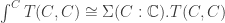
Here’s another nice thing about the theory of species in HoTT. In HoTT, coends whose index category are groupoids are just plain $\Sigma$ -types. That is, if $\mathbb{C}$ is a groupoid, $\mathbb{D}$ a category, and $T : \mathbb{C}^{\mathrm{op}} \times \mathbb{C} \to \mathbb{D}$ , then $\int^C T(C,C) \cong \Sigma (C : \mathbb{C}). T(C,C)$ . In set theory, this coend would be a quotient of the corresponding $\Sigma$ -type, but in HoTT the isomorphisms of $\mathbb{C}$ are required to correspond to paths, which automatically induce paths over the $\Sigma$ -type which correspond to the necessary quotient. Put another way, we can define coends in HoTT as a certain HIT, but in the case that $\mathbb{C}$ is a groupoid we already get all the paths given by the higher path constructor anyway, so it is redundant. So, what does this have to do with species, I hear you ask? Well, several species constructions involve coends (most notably partitional product); since species are functors from a groupoid, the definitions of these constructions in HoTT are particularly simple. We again get the right thing essentially “for free”.

There’s lots more in my dissertation, of course, but these are a few of the key ideas specifically relating species and HoTT. I am far from being an expert on either, but am happy to entertain comments, questions, etc. I can also point you to the right section of my dissertation if you’re interested in more detail about anything I mentioned above.

Parametricity and excluded middle

Exercise 6.9 of the HoTT book tells us that, and assuming LEM, we can exhibit a function $f:\Pi_{X:\mathcal{U}}(X\to X)$ such that $f_\mathbf{2}$ is a non-identity function $\mathbf{2}\to\mathbf{2}.$ I have proved the converse of this. Like in exercise 6.9, we assume univalence.

Parametricity

In a typical functional programming career, at some point one encounters the notions of parametricity and free theorems.

Parametricity can be used to answer questions such as: is every function

f : forall x. x -> x

equal to the identity function? Parametricity tells us that this is true for System F.

However, this is a metatheoretical statement. Parametricity gives properties about the terms of a language, rather than proving internally that certain elements satisfy some properties.

So what can we prove internally about a polymorphic function $f:\Pi_{X:\mathcal{U}}X\to X$ ?

In particular, we can see that internal proofs (claiming that $f$ must be the identity function for every type $X$ ) cannot exist: exercise 6.9 of the HoTT book tells us that, assuming LEM, we can exhibit a function $f:\Pi_{X:\mathcal{U}}(X\to X)$ such that $f_\mathbf{2}$ is $\mathsf{flip}:\mathbf{2}\to\mathbf{2}.$ (Notice that the proof of this is not quite as trivial as it may seem: LEM only gives us $P+\neg P$ if $P$ is a (mere) proposition (a.k.a. subsingleton). Hence, simple case analysis on $X\simeq\mathbf{2}$ does not work, because this is not necessarily a proposition.)

And given the fact that LEM is consistent with univalent foundations, this means that a proof that $f$ is the identity function cannot exist.

I have proved that LEM is exactly what is needed to get a polymorphic function that is not the identity on the booleans.

Theorem. If there is a function $f:\Pi_{X:\mathcal U}X\to X$ with $f_\mathbf2\neq\mathsf{id}_\mathbf2,$ then LEM holds.

Proof idea

If $f_\mathbf2\neq\mathsf{id}_\mathbf2,$ then by simply trying both elements $0_\mathbf2,1_\mathbf2:\mathbf2,$ we can find an explicit boolean $b:\mathbf2$ such that $f_\mathbf2(b)\neq b.$ Without loss of generality, we can assume $f_\mathbf2(0_\mathbf2)\neq 0_\mathbf2.$

For the remainder of this analysis, let $P$ be an arbitrary proposition. Then we want to achieve $P+\neg P,$ to prove LEM.

We will consider a type with three points, where we identify two points depending on whether $P$ holds. In other words, we consider the quotient of a three-element type, where the relation between two of those points is the proposition $P.$

I will call this space $\mathbf{3}_P,$ and it can be defined as $\Sigma P+\mathbf{1},$ where $\Sigma P$ is the suspension of $P.$ This particular way of defining the quotient, which is equivalent to a quotient of a three-point set, will make case analysis simpler to set up. (Note that suspensions are not generally quotients: we use the fact that $P$ is a proposition here.)

Notice that if $P$ holds, then $\mathbf{3}_P\simeq\mathbf{2},$ and also $(\mathbf{3}_P\simeq\mathbf{3}_P)\simeq\mathbf{2}.$

We will consider $f$ at the type $(\mathbf{3}_P\simeq\mathbf{3}_P)$ (not $\mathbf{3}_P$ itself!). Now the proof continues by defining

$g:=f_{\mathbf{3}_P\simeq\mathbf{3}_P}(\mathsf{ide}_{\mathbf{3}_P}):\mathbf{3}_P\simeq\mathbf{3}_P$

(where $\mathsf{ide_{\mathbf3_P}}$ is the equivalence given by the identity function on $\mathbf3_P$ ) and doing case analysis on $g(\mathsf{inr}(*)),$ and if necessary also on $g(\mathsf{inl}(x))$ for some elements $x:\Sigma P.$ I do not believe it is very instructive to spell out all cases explicitly here. I wrote a more detailed note containing an explicit proof.

Notice that doing case analysis here is simply an instance of the induction principle for $+.$ In particular, we do not require decidable equality of $\mathbf3_P$ (which would already give us $P+\neg P,$ which is exactly what we are trying to prove).

For the sake of illustration, here is one case:

$g(\mathsf{inr}(*))= \mathsf{inr}(*):$ Assume $P$ holds. Then since $(\mathbf{3}_P\simeq\mathbf{3}_P)\simeq\mathbf{2},$ then by transporting along an appropriate equivalence (namely the one that identifies $0_\mathbf2$ with $\mathsf{ide}_{\mathbf3_P}),$ we get $f_{\mathbf{3}_P\simeq\mathbf{3}_P}(\mathsf{ide}_{\mathbf{3}_P})\neq\mathsf{ide}_{\mathbf{3}_P}.$ But since $g$ is an equivalence for which $\mathsf{inr}(*)$ is a fixed point, $g$ must be the identity everywhere, that is, $g=\mathsf{ide}_{\mathbf{3}_P},$ which is a contradiction.

I formalized this proof in Agda using the HoTT-Agda library

Acknowledgements

Thanks to Martín Escardó, my supervisor, for his support. Thanks to Uday Reddy for giving the talk on parametricity that inspired me to think about this.

Colimits in HoTT

In this post, I would want to present you two things:

the small library about colimits that I formalized in Coq,
a construction of the image of a function as a colimit, which is essentially a sliced version of the result that Floris van Doorn talked in this blog recently, and further improvements.

I present my hott-colimits library in the first part. This part is quite easy but I hope that the library could be useful to some people. The second part is more original. Lets sketch it.
Given a function $f_0:\ A \rightarrow B$ we can construct a diagram

picture:iterated-diag1.png

where the HIT $\mathbf{KP}$ is defined by:

HIT KP f :=

| kp : A -> KP f

| kp_eq : forall x x', f(x) = f(x') -> kp(x) = kp(x').

and where $f_{n+1}$ is defined recursively from $f_n$ . We call this diagram the iterated kernel pair of $f_0$ . The result is that the colimit of this diagram is $\Sigma_{y:B} \parallel \mathbf{fib}_{f_0}\ y \parallel$ , the image of $f_0$ ( $\mathbf{fib}_{f_0}\ y$ is $\Sigma_{x:A}\ f_0(x) = y$ the homotopy fiber of $f_0$ in $y$ ).
It generalizes Floris’ result in the following sense: if we consider the unique arrow $f_0: A \rightarrow \mathbf{1}$ (where $\mathbf{1}$ is Unit) then $\mathbf{KP}(f_0)$ is $\{ A \}$ the one-step truncation of $A$ and the colimit is equivalent to $\parallel A \parallel$ the truncation of $A$ .

We then go further. Indeed, this HIT doesn’t respect the homotopy levels at all: even $\{\mathbf{1}\}$ is the circle. We try to address this issue considering an HIT that take care of already existing paths:

HIT KP' f :=

| kp : A -> KP' f

| kp_eq : forall x x', f(x) = f(x') -> kp(x) = kp(x').

| kp_eq_1 : forall x, kp_eq (refl (f x)) = refl (kp x)

This HIT avoid adding new paths when some elements are already equals, and turns out to better respect homotopy level: it at least respects hProps. See below for the details.
Besides, there is another interesting thing considering this HIT: we can sketch a link between the iterated kernel pair using $\mathbf{KP'}$ and the Čech nerve of a function. We outline this in the last paragraph.

All the following is joint work with Kevin Quirin and Nicolas Tabareau (from the CoqHoTT project), but also with Egbert Rijke, who visited us.

All our results are formalized in Coq. The library is available here:

https://github.com/SimonBoulier/hott-colimits

Colimits in HoTT

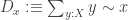
In homotopy type theory, Type, the type of all types can be seen as an ∞-category. We seek to calculate some homotopy limits and colimits in this category. The article of Jeremy Avigad, Krzysztof Kapulkin and Peter LeFanu Lumsdaine explain how to calculate the limits over graphs using sigma types. For instance an equalizer of two function $f$ and $g$ is $\Sigma_{x:A} f(x) = g(x)$ .
The colimits over graphs are computed in same way with Higher Inductive Types instead of sigma types. For instance, the coequalizer of two functions is

HIT Coeq (f g: A -> B) : Type :=

| coeq : B -> Coeq f g

| cp : forall x, coeq (f x) = coeq (g x).

In both case there is a severe restriction: we don’t know how two compute limits and colimits over diagrams which are much more complicated than those generated by some graphs (below we use an extension to “graphs with compositions” which is proposed in the exercise 7.16 of the HoTT book, but those diagrams remain quite poor).

We first define the type of graphs and diagrams, as in the HoTT book (exercise 7.2) or in hott-limits library of Lumsdaine et al.:

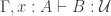
Record graph := {

G_0 :> Type ;

G_1 :> G_0 -> G_0 - Type }.

Record diagram (G : graph) := {

D_0 :> G -> Type ;

D_1 : forall {i j : G}, G i j -> (D_0 i -> D_0 j) }.

And then, a cocone over a diagram into a type $Q$ :

Record cocone {G: graph} (D: diagram G) (Q: Type) := {

q : forall (i: G), D i - X ;

qq : forall (i j: G) (g: G i j) (x: D i),

q j (D_1 g x) = q i x }.

Let $C:\mathrm{cocone}\ D\ Q$ be a cocone into $Q$ and $f$ be a function $Q \rightarrow Q'$ . Then we can extend $C$ to a cocone into $Q'$ by postcomposition with $f$ . It gives us a function

$\mathrm{postcompose} :\ (\mathrm{cocone}\ D\ Q) \rightarrow (Q': \mathrm{Type}) \rightarrow (Q \rightarrow Q')\rightarrow (\mathrm{cocone}\ D\ Q')$

picture:pict-colim.png

A cocone $C$ is said to be universal if, for all other cocone $C'$ over the same diagram, $C'$ can be obtained uniquely by extension of $C$ , that we translate by:

Definition is_universal (C: cocone D Q)

:= forall (Q': Type), IsEquiv (postcompose_cocone C Q').

Last, a type $Q$ is said to be a colimit of the diagram $D$ if there exists a universal cocone over $D$ into $Q$ .

Existence

The existence of the colimit over a diagram is given by the HIT:

HIT colimit (D: diagram G) : Type :=

| colim : forall (i: G), D i - colimit D

| eq : forall (i j: G) (g: G i j) (x: D i),

colim j (D_1 g x) = colim i x

Of course, $\mathrm{colimit}\ D$ is a colimit of $D$ .

Functoriality and Uniqueness

Diagram morphisms

Let $D$ and $D'$ be two diagrams over the same graph $G$ . A morphism of diagrams is defined by:

Record diagram_map (D1 D2 : diagram G) := {

map_0: forall i, D1 i - D2 i ;

map_1: forall i j (g: G i j) x,

D_1 D2 g (map_0 i x) = map_0 j (D_1 D1 g x) }.

We can compose diagram morphisms and there is an identity morphism. We say that a morphism $m$ is an equivalence of diagrams if all functions $m_i$ are equivalences. In that case, we can define the inverse of $m$ (reversing the proofs of commutation), and check that it is indeed an inverse for the composition of diagram morphisms.

Precomposition

We yet defined forward extension of a cocone by postcomposition, we now define backward extension. Given a diagram morphism $m: D \Rightarrow D'$ , we can make every cocone over $D'$ into a cocone over $D$ by precomposition by $m$ . It gives us a function

$\mathrm{precompose} :\ (D \Rightarrow D') \rightarrow (Q : \mathrm{Type})\rightarrow (\mathrm{cocone}\ D'\ Q) \rightarrow (\mathrm{cocone}\ D\ Q)$

picture:pict-precompose.png

We check that precomposition and postcomposition respect the identity and the composition of morphism. And then, we can show that the notions of universality and colimits are stable by equivalence.

Functoriality of colimits

Let $m: D \Rightarrow D'$ be a diagram morphism and $Q$ and $Q'$ two colimits of $D$ and $D'$ . Let’s note $C$ and $C'$ the universal cocone into $Q$ and $Q'$ . Then, we can get a function $Q \rightarrow Q'$ given by:

$(\mathrm{postcompose}\ C\ Q)^{-1}\ (\mathrm{precompose}\ m\ Q'\ C')$

We check that if $m$ is an equivalence of diagram then the function $Q' \rightarrow Q$ given by $m^{-1}$ is well an inverse of $Q \rightarrow Q'$ .
As a consequence, we get:

The colimits of two equivalents diagrams are equivalent.

Uniqueness

In particular, if we consider the identity morphism $D \Rightarrow D$ we get:

Let $Q_1$ and $Q_2$ be two colimits of the same diagram, then: $Q_1~\simeq~Q_2~$ .

So, if we assume univalence, the colimit of a diagram is truly unique!

Commutation with sigmas

Let $B$ be a type and, for all $y:B$ , $D^y$ a diagram over a graph $G$ . We can then build a new diagram over $G$ whose objects are the $\Sigma_y D_0^y(i)\$ and functions $\Sigma_y D_0^y(i) \rightarrow \Sigma_y D_0^y(j)$ are induced by the identity on the first component and by $D_1^y(g) : D_0^y(i) \rightarrow D_0^y(j)$ on the second one. Let’s note $\Sigma D$ this diagram.

Seemingly, from a family of cocone $C:\Pi_y\mathrm{cocone}\ D^y\ Q_y$ , we can make a cocone over $\Sigma D$ into $\Sigma_y Q_y$ .

picture:pict-sigma.png

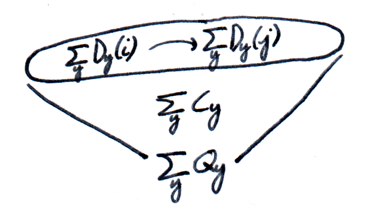
We proved the following result, which we believed to be quite nice:

If, for all $y:B\$ , $Q_y$ is a colimit of $D_y$ , then $\Sigma_y Q_y$ is a colimit of $\Sigma D$ .

Iterated Kernel Pair

First construction

Let’s first recall the result of Floris. An attempt to define the propositional truncation is the following:

HIT {_} (A: Type) :=

| α : A -> {A}

| e : forall (x x': A), α x = α x'.

Unfortunately, in general $\{ A \}$ is not a proposition, the path constructor $\mathrm{e}$ is not strong enough. But we have the following result:

Let $A$ be a type. Let’s consider the following diagram:
$A \rightarrow \{A\} \rightarrow \{\{A\}\} \rightarrow \dots$
Then, $\parallel A \parallel$ is a colimit of this diagram.

Let’s generalize this result to a function $f: A \rightarrow B$ (we will recover the theorem considering the unique function $A \rightarrow \mathbf{1}$ ).
Let $f: A \rightarrow B$ . We note $\mathbf{KP}(f)$ the colimit of the kernel pair of $f$ :

picture:diag-kp.png

where the pullback $A \times_B A$ is given by $\Sigma_{x,\, x'}\, f(x) = f(x')$ .
Hence, $\mathbf{KP}(f)$ is the following HIT:

Inductive KP f :=

| kp : A -> KP f

| kp_eq : forall x x', f(x) = f(x') -> kp(x) = kp(x').

Let’s consider the following cocone:

picture:cocone-kp.png

we get a function $\mathrm{lift}_f: \mathbf{KP}(f) \rightarrow B$ by universality (another point of view is to say that $\mathrm{lift}_f$ is defined by $\mathbf{KP\_rec}(f, \lambda\ p.\ p)$ ).

Then, iteratively, we can construct the following diagram:

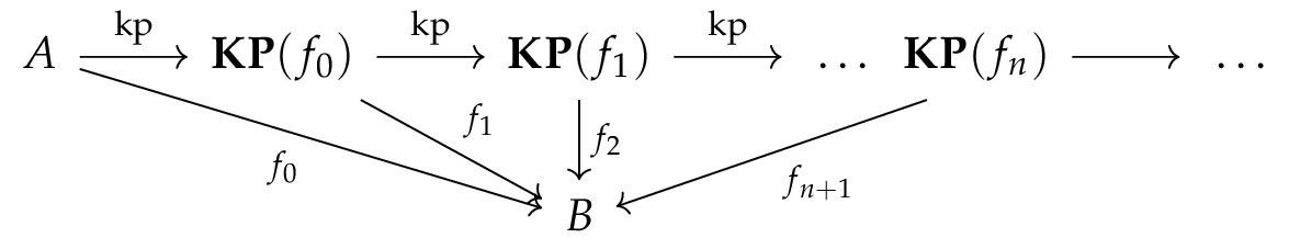
where $f_0 := f :\ A \rightarrow B$ and $f_{n+1} := \mathrm{lift}_{f_n} :\ \mathbf{KP}(f_n) \rightarrow B$ .
The iterated kernel pair of $f$ is the subdiagram

picture:iterated-diag1.png

We proved the following result:

The colimit of this diagram is 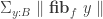$\Sigma_{y:B}\parallel \mathbf{fib}_f\ y\parallel \$ , the image of $f$ .

The proof is a slicing argument to come down to Floris’ result. It uses all properties of colimits that we talked above. The idea is to show that those three diagrams are equivalent.

Going from the first line to the second is just apply the equivalence $A\ \simeq\ \Sigma_{y:B}\mathbf{fib}_f\ y$ (for $f: A \rightarrow B$ ) at each type. Going from the second to the third is more involved, we don’t detail it here. And $\Sigma_{y:B}\parallel \mathbf{fib}_f\ y\parallel \$ is well the colimit of the last line: by commutation with sigmas it is sufficient to show that for all $y$ , $\parallel \mathbf{fib}_f\ y\parallel \$ is the colimit of the diagram

picture:diag-fib1.png

which is exactly Floris’ result!
The details are available here.

Second construction

The previous construction has a small defect: it did not respect the homotopy level at all. For instance $\{\mathbf{1}\}$ is the circle $\mathbb{S}^1$ . Hence, to compute $\parallel \mathbf{1}\parallel$ (which is $\mathbf{1}$ of course), we go through very complex types.

We found a way to improve this: adding identities!
Indeed, the proof keeps working if we replace $\mathbf{KP}$ by $\mathbf{KP'}$ which is defined by:

Inductive KP' f :=

| kp : A -> KP' f

| kp_eq : forall x x', f(x) = f(x') -> kp(x) = kp(x').

| kp_eq_1 : forall x, kp_eq (refl (f x)) = refl (kp x)

$\mathbf{KP'}$ can be seen as a “colimit with identities” of the following diagram :

picture:diag-kp-id1.png (♣)

with $\pi_i \circ \delta = \mathrm{id}$ .

In his article, Floris explains that, when $p:\ a =_A b$ then $\mathrm{ap}_\alpha(p)$ and $\mathrm{t\_eq}\ a\ b$ are not equal. But now they become equal: by path induction we bring back to $\mathrm{kp\_eq\_1}$ . That is, if two elements are already equal, we don’t add any path between them.
And indeed, this new HIT respects the homotopy level better, at least in the following sense:

$\mathbf{KP'}(\mathbf{1} \rightarrow \mathbf{1})$ is $\mathbf{1}$ (meaning that the one-step truncation of a contractible type is now $\mathbf{1}$ ),
If $f: A \rightarrow B$ is an embedding (in the sense that $\mathrm{ap}(f) : x = y \rightarrow f(x) = f(y)$ is an equivalence for all $x, y$ ) then so is $\mathrm{lift}_f : \mathbf{KP'}(f) \rightarrow B$ . In particular, if $A$ is hProp then so is $\mathbf{KP'}(A \rightarrow \mathbf{1})$ (meaning that the one-step truncation of an hProp is now itself).

Toward a link with the Čech nerve

Although we don’t succeed in making it precise, there are several hints which suggest a link between the iterated kernel pair and the Čech nerve of a function.
The Čech nerve of a function $f$ is a generalization of his kernel pair: it is the simplicial object

picture:diag-cech.png

(the degeneracies are not dawn but they are present).

We will call n-truncated Čech nerve the diagram restricted to the n+1 first objects:

picture:diag-cech-trunc.png

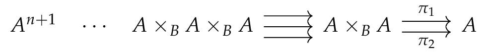
(degeneracies still here).

The kernel pair (♣) is then the 1-truncated Čech nerve.

We wonder to which extent $\mathbf{KP}(f_n)$ could be the colimit of the (n+1)-truncated Čech nerve. We are far from having such a proof but we succeeded in proving :

That $\mathbf{KP'}(f_0)$ is the colimit of the kernel pair (♣),
and that there is a cocone over the 2-trunated Čech nerve into $\mathbf{KP'}(f_1)$

(both in the sense of “graphs with compositions”, see exercise 7.16 of the HoTT book).

The second point is quite interesting because it makes the path concatenation appear. We don’t detail exactly how, but to build a cocone over the 2-trunated Čech nerve into a type $C$ , $C$ must have a certain compatibility with the path concatenation. $\mathbf{KP'}(f)$ doesn’t have such a compatibility: if $p:\ f(a) =_A f(b)$ and $q:\ f(b) =_A f(c)$ , in general we do not have

$\mathrm{kp\_eq}_f\ (p \centerdot q)\ =\ \mathrm{kp\_eq}_f\ p\ \centerdot\ \mathrm{kp\_eq}_f\ q$ in $\mathrm{kp}(a)\ =_{\mathbf{KP'}(f)}\ \mathrm{kp}(c)$ .

On the contrary, $\mathbf{KP'}(f_1)$ have the require compatibility: we can prove that

$\mathrm{kp\_eq}_{f_1}\ (p \centerdot q)\ =\ \mathrm{kp\_eq}_{f_1}\ p\ \centerdot\ \mathrm{kp\_eq}_{f_1}\ q$ in $\mathrm{kp}(\mathrm{kp}(a))\ =_{\mathbf{KP'}(f_1)}\ \mathrm{kp}(\mathrm{kp}(c))$ .

( $p$ has indeed the type $f_1(\mathrm{kp}(a)) = f_1(\mathrm{kp}(b))$ because $f_1$ is $\mathbf{KP\_rec}(f, \lambda\ p.\ p)$ and then $f_1(\mathrm{kp}(x)) \equiv x$ .)
This fact is quite surprising. The proof is basically getting an equation with a transport with apD and then making the transport into a path concatenation (see the file link_KPv2_CechNerve.v of the library for more details).

Questions

Many questions are left opened. To what extent $\mathbf{KP}(f_n)$ is linked with the (n+1)-truncated diagram? Could we use the idea of the iterated kernel pair to define a groupoid object internally? Indeed, in an ∞-topos every groupoid object is effective (by Giraud’s axioms) an then is the Čech nerve of his colimit…

The Lean Theorem Prover

Lean is a new player in the field of proof assistants for Homotopy Type Theory. It is being developed by Leonardo de Moura working at Microsoft Research, and it is still under active development for the foreseeable future. The code is open source, and available on Github.

You can install it on Windows, OS X or Linux. It will come with a useful mode for Emacs, with syntax highlighting, on-the-fly syntax checking, autocompletion and many other features. There is also an online version of Lean which you can try in your browser. The on-line version is quite a bit slower than the native version and it takes a little while to load, but it is still useful to try out small code snippets. You are invited to test the code snippets in this post in the on-line version. You can run code by pressing shift+enter.

In this post I’ll first say more about the Lean proof assistant, and then talk about the considerations for the HoTT library of Lean (Lean has two libraries, the standard library and the HoTT library). I will also cover our approach to higher inductive types. Since Lean is not mature yet, things mentioned below can change in the future.

Update January 2017: the newest version of Lean currently doesn’t support HoTT, but there is a frozen version which does support HoTT. The newest version is available here, and the frozen version is available here. To use the frozen version, you will have to compile it from the source code yourself.

Continue reading →

Real-cohesive homotopy type theory

Two new papers have recently appeared online:

Both of them have fairly chatty introductions, so I’ll try to restrain myself from pontificating at length here about their contents. Just go read the introductions. Instead I’ll say a few words about how these papers came about and how they are related to each other.

Continue reading →

A new class of models for the univalence axiom

First of all, in case anyone missed it, Chris Kapulkin recently wrote a guest post at the n-category cafe summarizing the current state of the art regarding “homotopy type theory as the internal language of higher categories”.

I’ve just posted a preprint which improves that state a bit, providing a version of “Lang(C)” containing univalent strict universes for a wider class of (∞,1)-toposes C:

Univalence for inverse EI diagrams

Continue reading →

Constructing the Propositional Truncation using Nonrecursive HITs

In this post, I want to talk about a construction of the propositional truncation of an arbitrary type using only non-recursive HITs. The whole construction is formalized in the new proof assistant Lean, and available on Github. I’ll write another blog post explaining more about Lean in August.

Continue reading →

Universal Properties of Truncations

Some days ago at the HoTT/UF workshop in Warsaw (which was a great event!), I have talked about functions out of truncations. I have focussed on the propositional truncation $\Vert - \Vert$ , and I want to write this blog post in case someone could not attend the talk but is interested nevertheless. There are also my slides and the arXiv paper.
The topic of my talk can be summarised as

Question: What is the type $\Vert A \Vert \to B$ ?

This question is very easy if $B$ is propositional, because then we have

Partial answer (1): If $B$ is propositional, then $(\Vert A \Vert \to B) \simeq (A \to B)$

by the usual universal property, with the equivalence given by the canonical map. Without an assumption on $B$ , it is much harder.

The rest of this post contains a special case which already contains some of the important ideas. It is a bit lengthy, and in case you don’t have time to read everything, here is the

Main result (general universal property of the propositional truncation).
In a dependent type theory with at least $\mathbf{1}$ , $\Sigma$ -, $\Pi$ -, and identity types, which furthermore has Reedy $\omega^{\mathsf{op}}$ -limits (“infinite $\Sigma$ -types”), we can define the type of coherently constant functions $A \xrightarrow {\omega} B$ as the type of natural transformations between type-valued presheaves. If the type theory has propositional truncations, we can construct a canonical map from $\Vert A \Vert \to B$ to $A \xrightarrow {\omega} B$ . If the type theory further has function extensionality, then this canonical map is an equivalence.
If $B$ is known to be $n$ -truncated for some fixed $n$ , we can drop the assumption of Reedy $\omega^{\mathsf{op}}$ -limits and perform the whole construction in “standard syntactical” HoTT. This describes how functions $\Vert A \Vert \to B$ can be defined if $B$ is not known to be propositional, and it streamlines the usual approach of finding a propositional $Q$ with $A \to Q$ and $Q \to B$ .

Here comes the long version of this blog post. So, what is a function $g : \Vert A \Vert \to B$ ? If we think of elements of $\Vert A \Vert$ as anonymous inhabitants of $A$ , we could expect that such a $g$ is “the same” as a function $f : A \to B$ which “cannot look at its input”. But then, how can we specify what it means to “not look at its input” internally? A first attempt could be requesting that $f$ is weakly constant, $\mathsf{wconst}_f :\equiv \Pi_{x,y:A} f(x) = f(y)$ . Indeed, it has been shown:

Partial answer (2): If $B$ is a set (h-set, $0$ -truncated), then $(\Vert A \Vert \to B) \simeq (\Sigma (f : A \to B). \mathsf{wconst}_f)$ , where the function from left to right is the canonical one.

It is not surprising that we still need this strong condition on $B$ if we want weak constancy to be a sufficient answer: just throwing in a bunch of paths, which might or might not “fit together” (we just don’t know anything) seems wrong. Indeed, from Mike’s recent construction, we know that the statement does become false (contradicts univalence) without this requirement.

Given a function $f : A \to B$ and a proof $c : \mathsf{wconst}_f$ , we can try to fix the problem that the paths given by $c$ “do not fit together” by throwing in a coherence proof, i.e. an element of $\mathsf{coh}_{f,c} :\equiv \Pi_{x,y,z:A} c(x,y) \cdot c(y,z) = c(x,z)$ . We should already know that this will introduce its own problems and thus not fix everything, but at least, we get:

Partial answer (3): If $B$ is $1$ -truncated, then $(\Vert A \Vert \to B) \simeq (\Sigma (f : A \to B). \Sigma (c:\mathsf{wconst}_f). \mathsf{coh}_{f,c})$ , again given by a canonical map from left to right.

In my talk, I have given a proof of “partial answer (3)” via “reasoning with equivalences” (slides p. 5 ff). I start by assuming a point $a_0 : A$ . The type $B$ is then equivalent to the following (explanation below):

$\Sigma (f_1 : B).$
$\Sigma (f : A \to B). \Sigma (c_1 : \Pi_{a:A} f(a) = f_1).$
$\Sigma (c : \mathsf{const}_f). \Sigma(d_1 : \Pi_{a^1, a^2:A} c(a^1,a^2) \cdot c_1(a^2) = c_1(a^1)$
$\Sigma (c_2 : f(a_0) = f_1). \Sigma (d_3 : c(a_0,a_0) \cdot c_1(a_0) = c_2).$
$\Sigma (d : \mathsf{coh}_{f,c_0}).$
$\Sigma (d_2 : \Pi_{a:A} c(a_0,a) \cdot c_1(a) = c_2).$
$\mathbf{1}$

In the above long nested $\Sigma$ -type, the first line is just the $B$ that we start with. The second line adds two factors/ $\Sigma$ -components which, by function extensionality, cancel each other out (they form a singleton). The same is true for the pair in the third line, and for the pair in the fourth line. Lines five and six look different, but they are not really; it’s just that their “partners” (which would complete them to singletons) are hard to write down and, at the same time, contractible; thus, they are omitted. As $B$ is assumed to be a $1$ -type, it is easy to see that the $\Sigma$ -components in lines five and six are both propositional, and it’s also easy to see that the other $\Sigma$ -components imply that they are both inhabited. Of course, the seventh line does nothing.

Simply by re-ordering the $\Sigma$ -components in the above type, and not doing anything else, we get:

$\Sigma (f : A \to B). \Sigma(c : \mathsf{const}_f). \Sigma(d : \mathsf{coh}_{f,c}).$
$\Sigma (f_1 : B) \Sigma(c_2 : f(a_0) = f_1).$
$\Sigma (c_1 : \Pi_{a:A} f(a) = f_1). \Sigma(d_2 : \Pi_{a:A} c(a_0,a) \cdot c_1(a) = c_2).$
$\Sigma (d_1 : \Pi_{a^1, a^2:A} c(a^1,a^2) \cdot c_1(a^2) = c_1(a^1)).$
$\Sigma (d_3 : c(a_0,a_0) \cdot c_1(a_0) = c_2).$
$\mathbf{1}$

By the same argument as before, the components in the pair in line two cancel each other out (i.e. the pair is contractible). The same is true for line three. Line four and five are propositional as $B$ is $1$ -truncated, but easily seen to be inhabited. Thus, the whole nested $\Sigma$ -type is equivalent to $\Sigma (f : A \to B). \Sigma(c : \mathsf{const}_f). \mathsf{coh}_{f,c}$ .
In summary, we have constructed an equivalence $B \simeq \Sigma (f : A \to B). \Sigma(c : \mathsf{const}_f). \mathsf{coh}_{f,c}$ . By going through the construction step-by-step, we see that the function part of the equivalence (map from left to right) is the canonical one (let’s write $\mathsf{canon}_1$ ), mapping $b : B$ to the triple $(\lambda \_. b, \lambda \_ \_ . \mathsf{refl}_b , \lambda \_ \_ \_ . \mathsf{refl}_{\mathsf{refl}_b})$ . Before we have started the construction, we have assumed a point $a_0 : A$ . But, and this is the crucial observation, the function $\mathsf{canon}_1$ does not depend on $a_0$ ! So, if the assumption $A$ implies that $\mathsf{canon}_1$ is an equivalence, then $\Vert A \Vert$ is already enough. Thus, we have $\Vert A \Vert \to \big(B \simeq \Sigma (f : A \to B). \Sigma(c : \mathsf{const}_f). \mathsf{coh}_{f,c}\big)$ . We can move the $\Vert A \Vert \to$ -part to both sides of the equivalence, and on the right-hand side, we can apply the usual “distributivity of $\Sigma$ and $\Pi$ (or $\to$ )”, to move the $\Vert A \Vert \to$ into each $\Sigma$ -component; but in each $\Sigma$ -component, the $\Vert A \Vert$ gets eaten by an $A$ (we have that $\Vert A \Vert \to \Pi_{a : A}\ldots$ and $\Pi_{a:A} \ldots$ are equivalent), which gives us the claimed result.

The strategy we have used is very minimalistic. It does not need any “technology”: we just add and remove contractible pairs. For this “expanding and contracting” strategy, we have really only used very basic components of type theory ( $\Sigma$ , $\Pi$ , identity types with function extensionality, propositional truncation, but even that only in the very end). If we want to weaken the requirement on $B$ by one more level (i.e. if we want to derive a “universal property” which characterises $\Vert A \Vert \to B$ if $B$ is $2$ -truncated), we have to add one more coherence condition (which ensures that the $\mathsf{coh}_{f,c}$ -component is well-behaved). The core idea is that this expanding and contracting strategy can be done for any truncation level of $B$ , even if $B$ is not known to be $n$ -truncated at all, where the tower of conditions becomes infinite. I call an element of this “infinite $\Sigma$ -type” a coherently constant function from $A$ to $B$ .

The idea is that the $\Sigma$ -components $(f : A \to B)$ and $(c : \mathsf{const}_f)$ and $(d : \mathsf{coh}_{f,c})$ we used in the special case can be seen as components of a natural transformation between $[2]$ -truncated semi-simplicial types. By semi-simplicial type, I mean a Reedy fibrant diagram $\Delta_+^{\mathsf{op}} \to \mathcal{C}$ . By $[2]$ -truncated semi-simplicial types, I mean the “initial segments” of semi-simplicial types, the first three components $X_0, X_1, X_2$ as described here.
The first diagram we need is what I call the “trivial semi-simplicial type” over $A$ , written $T \! A$ , and its initial part is given by $T \! A_{[0]} :\equiv A$ , $T \! A_{[1]} :\equiv A \times A$ , and $T \! A_{[2]} :\equiv A \times A \times A$ . If we use the “fibred” notation (i.e. give the fibres over the matching objects), this would be $T \! A_{[0]} :\equiv A$ , $T \! A_{[1]}(a_1,a_2) :\equiv \mathbf{1}$ , $T \! A_{[2]}(a_1,a_2,a_3,\_,\_,\_) :\equiv \mathbf{1}$ . In the terminology of simplicial sets, this is the $[0]$ -coskeleton of [the diagram that is constantly] $A$ .
The second important diagram, I call it the equality semi-simplicial type over $B$ , is written $E \! B$ . One potential definition for the lowest levels would be given by (I only give the fibres this time): $E \! B_{[0]} :\equiv B$ , $E \! B_{[1]}(b_1,b_2) :\equiv b_1 = b_2$ , $E \! B_{[2]}(b_1,b_2,b_3,p_{12},p_{23},p_{13}) :\equiv p_{12} \cdot p_{23} = p_{13}$ . This is a fibrant replacement of $B$ . (We are lucky because $T \! A$ is already fibrant; otherwise, we should have constructed a fibrant replacement as well.)
If we now check what a (strict) natural transformation between $T \! A$ and $E \! B$ (viewed as diagrams over the full subcategory of $\Delta_+^{\mathsf{op}}$ with objects $[0],[1],[2]$ ) is, it is easy to see that the $[0]$ -component is exactly a map $f : A \to B$ , the $[1]$ -component is exactly a proof $c : \mathsf{const}_f$ , and the $[2]$ -component is just a proof $d : \mathsf{coh}_{f,c}$ . (The type of such natural transformations is given by the limit of the exponential of $T \! A$ and $E \! B$ .)

However, even with this idea, and with the above proof for the case that $B$ is $1$ -truncated, generalising this proof to the infinite case with infinitely many coherence conditions requires some ideas and a couple of technical steps which, for me, have been quite difficult. Therefore, it has taken me a very long time to write this up cleanly in an article. I am very grateful to the reviewers (this work is going to appear in the post-proceedings of TYPES’14) and to Steve (my thesis examiner) for many suggestions and interesting connections they have pointed out. In particular, one reviewer has remarked that the main result (the equivalence of coherently constant functions $A \xrightarrow{\omega} B$ and maps out of the truncation $\Vert A \Vert \to B$ ) is a type-theoretic version of Proposition 6.2.3.4 in Lurie’s Higher Topos Theory; and Vladimir has pointed out the connection to the work of his former student Alexander Vishik. Unfortunately, both are among the many things that I have yet to understand, but there is certainly a lot to explore. If you can see further connections which I have not mentioned here or in the paper, then this is very likely because I am not aware of them, and I’d be happy to hear about it!

Modules for Modalities

As defined in chapter 7 of the book, a modality is an operation on types that behaves somewhat like the n-truncation. Specifically, it consists of a collection of types, called the modal ones, together with a way to turn any type $A$ into a modal one $\bigcirc A$ , with a universal property making the modal types a reflective subcategory (or more precisely, sub-(∞,1)-category) of the category of all types. Moreover, the modal types are assumed to be closed under Σs (closure under some other type formers like Π is automatic).

We called them “modalities” because under propositions-as-(some)-types, they look like the classical notion of a modal operator in logic: a unary operation on propositions. Since these are “monadic” modalities — in particular, we have $A \to \bigcirc A$ rather than the other way around — they are most closely analogous to the “possibility” modality of classical modal logic. But since they act on all types, not just mere-propositions, for emphasis we might call them higher modalities.

The example of n-truncation shows that there are interesting new modalities in a homotopy world; some other examples are mentioned in the exercises of chapter 7. Moreover, most of the basic theory of n-truncation — essentially, any aspect of it that involves only one value of n — is actually true for any modality.

Over the last year, I’ve implemented this basic theory of modalities in the HoTT Coq library. In the process, I found one minor error in the book, and learned a lot about modalities and about Coq. For instance, my post about universal properties grew out of looking for the best way to define modalities.

In this post, I want to talk about something else I learned about while formalizing modalities: Coq’s modules, and in particular their universe-polymorphic nature. (This post is somewhat overdue in that everything I’ll be talking about has been implemented for several months; I just haven’t had time to blog about it until now.)

Continue reading →

Not every weakly constant function is conditionally constant

As discussed at length on the mailing list some time ago, there are several different things that one might mean by saying that a function $f:A\to B$ is “constant”. Here is my preferred terminology:

$f$ is constant if we have $b:B$ such that $f(a)=b$ for all $a:A$ .
This is equivalent to saying that $f$ factors through $\mathbf{1}$ .
$f$ is conditionally constant if it factors through $\Vert A \Vert$ .
$f$ is weakly constant if for all $a_1,a_2:A$ we have $f(a_1)=f(a_2)$ .

In particular, the identity function of $\emptyset$ is conditionally constant, but not constant. I don’t have a problem with that; getting definitions right often means that they behave slightly oddly on the empty set (until we get used to it). The term “weakly constant” was introduced by Kraus, Escardo, Coquand, and Altenkirch, although they immediately dropped the adjective for the rest of their paper, which I will not do. The term “conditionally constant” is intended to indicate that $f$ is, or would be, constant, as soon as its domain is inhabited.

It’s obvious that every constant function is conditionally constant, and $\mathrm{id}_{\emptyset}$ shows the converse fails. Similarly, it’s easy to show that conditionally constant implies weakly constant. KECA showed that the converse holds if either $B$ is a set or $\Vert A \Vert \to A$ , and conjectured that it fails in general. In this post I will describe a counterexample proving this conjecture.

Continue reading →

Double Groupoids and Crossed Modules in HoTT

The past eight months I spent at CMU for my master thesis project. I ended up formalizing some algebraic structures used in Ronald Brown’s book “Non-Abelian Algebraic Topology”: Double groupoids with thin structure and crossed modules over groupoids.

As the language for the formalizations I chose the newly developed theorem prover Lean. Lean is developed by Leonardo de Moura at Microsoft Research and provides a dependently typed language similar to Agda or Coq. Currently, there are two modes for Lean: A proof-irrelevant mode and a HoTT mode. The HoTT library was written at the same time as my project, mainly by Floris van Doorn and, for a smaller part, me. You can find papers about Lean and its elaboration algorithm on the website, as well as a link to a version of Lean that runs in your web browser.

Double groupoids are a special case double categories which, besides objects and morphisms, specify a set of two-cells for each (not necessarily commuting) square diagram in a way such that the two-cells form a category with respect to vertical and to horizontal composition. That includes the existence of vertically and horizontally degenerate fillers of square diagrams with the identity on two opposing sides and the same morphism on the other side. The vertically degenerate squares should distribute over the horizontal composition of morphisms and vice versa. Furthermore, the vertically and horizontally degenerate square along the identity should be the same. A last axiom is the interchange law which ensures that, in the case of two-cells which are composable in a 2×2-grid, it doesn’t matter whether to first compose vertically or horizontally.

I decided to formalize double categories in the same way categories are usually formalized using dependent types using a type of two-cells depending on four points and four morphisms:

$D_2 : \prod_{a, b, c, d : D_0} \text{hom}(a,b) \to \text{hom}(c,d) \to \text{hom}(a,c) \to \text{hom}(b,d) \to \mathcal{U}.$ In the formalization, I first define a worm precategory which only allows for two-cell composition in one direction. Then, I use Lean’s inheritance mechanism to get the full notion of a double (pre)category:

structure worm_precat {D₀ : Type} (C : precategory D₀)

(D₂ : Π ⦃a b c d : D₀⦄

(f : hom a b) (g : hom c d) (h : hom a c) (i : hom b d), Type) :=

(comp₁ : proof Π ⦃a b c₁ d₁ c₂ d₂ : D₀⦄

⦃f₁ : hom a b⦄ ⦃g₁ : hom c₁ d₁⦄ ⦃h₁ : hom a c₁⦄ ⦃i₁ : hom b d₁⦄

⦃g₂ : hom c₂ d₂⦄ ⦃h₂ : hom c₁ c₂⦄ ⦃i₂ : hom d₁ d₂⦄,

(D₂ g₁ g₂ h₂ i₂) → (D₂ f₁ g₁ h₁ i₁)

→ (@D₂ a b c₂ d₂ f₁ g₂ (h₂ ∘ h₁) (i₂ ∘ i₁)) qed)

(ID₁ : proof Π ⦃a b : D₀⦄ (f : hom a b), D₂ f f (ID a) (ID b) qed)

(assoc₁ : proof Π ⦃a b c₁ d₁ c₂ d₂ c₃ d₃ : D₀⦄

⦃f : hom a b⦄ ⦃g₁ : hom c₁ d₁⦄ ⦃h₁ : hom a c₁⦄ ⦃i₁ : hom b d₁⦄

⦃g₂ : hom c₂ d₂⦄ ⦃h₂ : hom c₁ c₂⦄ ⦃i₂ : hom d₁ d₂⦄

⦃g₃ : hom c₃ d₃⦄ ⦃h₃ : hom c₂ c₃⦄ ⦃i₃ : hom d₂ d₃⦄

(w : D₂ g₂ g₃ h₃ i₃) (v : D₂ g₁ g₂ h₂ i₂) (u : D₂ f g₁ h₁ i₁),

(assoc i₃ i₂ i₁) ▹ ((assoc h₃ h₂ h₁) ▹

(comp₁ w (comp₁ v u))) = (comp₁ (comp₁ w v) u) qed)

...

structure dbl_precat {D₀ : Type} (C : precategory D₀)

(D₂ : Π ⦃a b c d : D₀⦄

(f : hom a b) (g : hom c d) (h : hom a c) (i : hom b d), Type)

extends worm_precat C D₂,

worm_precat C (λ ⦃a b c d : D₀⦄ f g h i, D₂ h i f g)

renaming comp₁→comp₂ ID₁→ID₂ assoc₁→assoc₂

id_left₁→id_left₂ id_right₁→id_right₂ homH'→homH'_dontuse :=

...

(interchange : proof Π {a₀₀ a₀₁ a₀₂ a₁₀ a₁₁ a₁₂ a₂₀ a₂₁ a₂₂ : D₀}

{f₀₀ : hom a₀₀ a₀₁} {f₀₁ : hom a₀₁ a₀₂} {f₁₀ : hom a₁₀ a₁₁}

{f₁₁ : hom a₁₁ a₁₂} {f₂₀ : hom a₂₀ a₂₁} {f₂₁ : hom a₂₁ a₂₂}

{g₀₀ : hom a₀₀ a₁₀} {g₀₁ : hom a₀₁ a₁₁} {g₀₂ : hom a₀₂ a₁₂}

{g₁₀ : hom a₁₀ a₂₀} {g₁₁ : hom a₁₁ a₂₁} {g₁₂ : hom a₁₂ a₂₂}

(x : D₂ f₁₁ f₂₁ g₁₁ g₁₂) (w : D₂ f₁₀ f₂₀ g₁₀ g₁₁)

(v : D₂ f₀₁ f₁₁ g₀₁ g₀₂) (u : D₂ f₀₀ f₁₀ g₀₀ g₀₁),

comp₁ (comp₂ x w) (comp₂ v u) = comp₂ (comp₁ x v) (comp₁ w u) qed)

Double groupoids are double categories where all three categories involved — the underlying category of points and morphisms, the vertical category of two-cells, and the horizontal category of two-cells — are groupoids and that are equipped with a thin structure: A selection of a unique thin filler of each commutative square shell which is closed under composition and degenerate squares.

It turns out that a category equivalent to the one of double groupoids is the category of crossed modules over a groupoid. A crossed module is defined as a groupoid $P$ together with a family $(M_p)_{p \in P}$ of groups (or, equivalently, a totally disconnected groupoid) on the objects of $P$ and for each $p \in P$ a group homomorphism $\mu_p : M_p \to \text{hom}(p,p)$ and a groupoid action $\phi$ of $P$ on the $(M_p)_{p \in P}$ . The family of homomorphisms and the action should interact by resembling conjugation via $\mu_q(\phi(f,x)) = f \circ \mu_p(x) \circ f^{-1}$ and $\phi(\mu_p(c),x) = c \cdot x \cdot c^{-1}$ for each $p, q \in P$ , $f \in \text{hom}_P(p,q)$ and $c, x \in M_p$ .

structure xmod {P₀ : Type} [P : groupoid P₀] (M : P₀ → Group) :=

(P₀_hset : is_hset P₀)

(μ : Π ⦃p : P₀⦄, M p → hom p p)

(μ_respect_comp : Π ⦃p : P₀⦄ (b a : M p), μ (b * a) = μ b ∘ μ a)

(μ_respect_id : Π (p : P₀), μ 1 = ID p)

(φ : Π ⦃p q : P₀⦄, hom p q → M p → M q)

(φ_respect_id : Π ⦃p : P₀⦄ (x : M p), φ (ID p) x = x)

(φ_respect_P_comp : Π ⦃p q r : P₀⦄ (b : hom q r) (a : hom p q) (x : M p),

φ (b ∘ a) x = φ b (φ a x))

(φ_respect_M_comp : Π ⦃p q : P₀⦄ (a : hom p q) (y x : M p),

φ a (y * x) = (φ a y) * (φ a x))

(CM1 : Π ⦃p q : P₀⦄ (a : hom p q) (x : M p), μ (φ a x) = a ∘ (μ x) ∘ a⁻¹)

(CM2 : Π ⦃p : P₀⦄ (c x : M p), φ (μ c) x = c * (x * c⁻¹ᵍ))

After formlizing both categories, DGpd and Xmod including the definition of their respective morphisms, I defined the functors $\gamma$ and $\lambda$ which establish their equivalence.

definition gamma.functor :

functor Cat_dbl_gpd.{l₁ l₂ l₃} Cat_xmod.{(max l₁ l₂) l₂ l₃} :=

begin

fapply functor.mk,

intro G, apply (gamma.on_objects G),

intros [G, H, F], apply (gamma.on_morphisms F),

intro G, cases G,

fapply xmod_morphism_congr, apply idp, apply idp,

repeat ( apply eq_of_homotopy ; intros), cases x_1, apply idp,

...

end

Since establishing the functors was quite tedious, I didn’t finish proving the equivalence, but I might do that in the future.

As a little application on 2-types I instantiated the fundamental double groupoid of a 2-type $X$ which is presented by a set $C$ and a 1-type $A$ by arbitrary functions $\iota : C \to A$ and $\iota' : A \to X$ . Here, the type of objects is the set $C$ , the set of morphisms between $a, b : C$ is the identity type $\iota(a) =_A \iota(b)$ , and the set of two-cells associated to four points $a, b, c, d : C$ and paths $f, g, h, i$ on the top, bottom, left and right of a diagram is the set $\text{ap}_{\iota'}(h) \cdot \text{ap}_{\iota'}(g) = \text{ap}_{\iota'}(f) \cdot \text{ap}_{\iota'}(i)$ . This could serve as the starting point to formalize a 2-dimensional Seifert-van Kampen theorem using double groupoids or crossed modules.

You can find my thesis here. The Lean code used can be found on github, due to recent changes in Lean, it most probably won’t compile with the newest version of Lean but with an older snapshot that can be found here.

The torus is the product of two circles, cubically

Back in the summer of 2012, emboldened by how nicely the calculation π₁(S¹) had gone, I asked a summer research intern, Joseph Lee, to work on formalizing a proof that the higher-inductive definition of the torus (see Section 6.6 of the HoTT book) is equivalent to a product of two circles. This seemed to me like it should be a simple exercise: define the functions back and forth by recursion, and then prove that they’re mutually inverse by induction. Joseph and I managed to define the two functions, but after spending a while staring at pages-long path algebra goals in both Agda and Coq, we eventually threw in the towel on proving that they were mutually inverse. By the end of the IAS year, both Kristina Sojakova and Peter Lumsdaine had given proof sketches, and Kristina’s later appeared as a 25-page proof in the exercise solutions of the book. But it still bothered me that we didn’t have a simple proof of what seemed like it should be a simple theorem…

Since the Bezem, Coquand, and Huber cubical sets model of HoTT was developed, Guillaume Brunerie and I have been thinking about cubical type theories based on these ideas (more on that in some other post). As part of this, we have also played with using cubical ideas in “book HoTT” (MLTT with axioms for univalence and HITs) in Agda. The main ingredient is to make use of more general “cube types” than just the identity type (the special case of lines). Each cube type is dependent on the boundary of a cube, and represents the “inside” of the boundary. For example, we have a type of squares, dependent on four points and four paths that make up the boundary of a square. And a type of cubes, dependent on the eight points, twelve lines, and six squares that make up the boundary of a cube (implicit arguments are crucial here: everything but the squares can be implicit). Another ingredient is to use path-over-a-path and higher cube-over-a-cube types to represent paths in fibrations.

Now, these cube types are not really “new”, in the sense that they can be defined in terms of higher identity types. For example, a square can be represented by a disc between composites, and a path-over can be reduced to homogeneous paths using transport. However, isolating these cubes and cube-overs as abstractions, and developing some facts about them, has allowed for the formalization of some new examples. Guillaume used this approach to prove the 3×3 lemma about pushouts that is used in the calculation of the Hopf fibration. I used it to resolve a question about the contractibility of a patch theory. Evan Cavallo used it in the proof of the Mayer-Vietoris theorem.

And, we finally have a simple write-the-maps-back-and-forth-and-then-induct-and-beta-reduce proof that the torus is a product of two circles.

You can read about it here:

A Cubical Approach to Synthetic Homotopy Theory
Daniel R. Licata and Guillaume Brunerie

Homotopy theory can be developed synthetically in homotopy type theory, using types to describe spaces, the identity type to describe paths in a space, and iterated identity types to describe higher-dimensional paths. While some aspects of homotopy theory have been developed synthetically and formalized in proof assistants, some seemingly straightforward examples have proved difficult because the required manipulations of paths becomes complicated. In this paper, we describe a cubical approach to developing homotopy theory within type theory. The identity type is complemented with higher-dimensional cube types, such as a type of squares, dependent on four points and four lines, and a type of three-dimensional cubes, dependent on the boundary of a cube. Path-over-a-path types and higher generalizations are used to describe cubes in a fibration over a cube in the base. These higher-dimensional cube and path-over types can be defined from the usual identity type, but isolating them as independent conceptual abstractions has allowed for the formalization of some previously difficult examples.

HoTT is not an interpretation of MLTT into abstract homotopy theory

Almost at the top of the HoTT website are the words:

“Homotopy Type Theory refers to a new interpretation of Martin-Löf’s system of intensional, constructive type theory into abstract homotopy theory. ”

I think it is time to change these words into something that, at least, is not wrong.

Is there an interpretation of the MLTT into abstract homotopy theory? This would be the case if the 2007/2009 paper by Awodey and Warren defined, as it is often claimed today, an interpretation of MLTT into any Quillen model category.

However, that paper did not provide a construction of any interpretation of the MLTT . It outlined several ideas connecting the factorization axioms of Quillen model categories with the introduction and elimination rules for the identity types in the intensional Martin-Lof Type Theory. These ideas did not quite work out because the operations that one can define on a general Quillen model category do not satisfy the relations that are present in the MLTT .

Using an analogy from the representation theory, they noticed that there is a similarity between the generators of a certain “group” (MLTT) and operations in some categories. This would define representations of the group in such categories but it turned out that one of the most important relations in the group did not hold in the categories. The paper claimed (without a proof) that there is a new “group” that they called “a form of MLTT” that did not have this relation in its definition and stated the main result by saying that “there is an interpretation of a form of MLTT in any Quillen model category”.

The truth concerning the interpretations of MLTT into homotopy theory is different.

1. No interpretation of the MLTT into abstract homotopy theory (general Quillen model category) is known. Moreover, it is unreasonable to expect such an interpretation to exist if only because not every Quillen model category is locally cartesian closed. For example, the category of complexes of abelian groups is a Quillen model category that is not even cartesian closed.

2. The interpretation of the rules for identity types on model categories from a class that contains such important examples as topological spaces and simplicial sets was constructed in a 2008/2012 paper by Benno van den Berg and Richard Garner.

3. An interpretation of the rules for the dependent products, dependent sums, identity types and universes on the category of simplicial sets was constructed by Vladimir Voevodsky in 2009. The outline of the construction was made publicly available in the early 2010 and then written up in a 2012 paper by Chris Kapulkin, Peter LeFanu Lumsdaine and Vladimir Voevodsky.

There is a substantial difficulty in adding the rules for universes to the rules for the dependent products, dependent sums and identity types. These three groups of rules are independent from each other and can be studied separately. The rules for a universe connect the rules from these three groups to each other making it necessary to coordinate their interpretations.

4. An interpretation of the the same complement of rules on the categories of special diagrams of simplicial sets was constructed in 2012/13 by Michael Shulman. This was an important advance since it proved that an interpretation of these rules that satisfy the univalence axiom need not satisfy the excluded middle property.

The results mentioned above all provide interpretation of the various *rules* of the MLTT not of the MLTT itself.

MLTT is a syntactic object. Its definition starts with a specification of the “raw” syntax. Then one considers four sets that consist of all the sentences of four standard shapes that can be written in this syntax. Then, one takes the smallest quadruple of subsets of these sets that is closed under certain operations (the “rules”). Then one performs an extra step of taking the quotient of the two of the resulting sets by equivalences relations determined by the other two sets.

At this point one is left with two sets and a number of operations on these two sets. From this structure one constructs, using yet another procedure, a category. This category is called the syntactic category of the MLTT.

An interpretation of the MLTT is a functor from the syntactic category to another category.

There is a way to define interpretation of the rules of the MLTT on any category with some additional structure. It is a long standing conjecture that the syntactic category of the MLTT is the initial object among categories where the interpretation of the rules of the MLTT is given.

This conjecture is far from being proved.

In a remarkable 1991 book by Thomas Streicher proved an analog of this conjecture for a much more simple type theory called the Calculus of Constructions (not to be confused with the Calculus of Inductive Constructions!). At the moment it remains to be the only substantially non-trivial analog of this conjecture known.

Until this conjecture is proved, all of the previous papers can only claim interpretation of the rules of the MLTT not an interpretation of the MLTT. Proving this conjecture in a way that will also enable us to prove its analogs for yet more complex type theories such as the Calculus of Inductive Constructions and its extensions with new classes of inductive types is the most important, from my point of view, goal that needs to be achieved in the development of the UF and HoTT.

The HoTT Book does not define HoTT

The intent of this post is to address certain misconceptions that I’ve noticed regarding the HoTT Book and its role in relation to HoTT. (At least, I consider them misconceptions.) Overall, I think the HoTT Book project has been successful beyond the dreams of the authors, both in disseminating the ideas of the subject to a wide audience, and in serving as a reference for further work. But perhaps because of that very success, it’s easy for people to get the impression that the HoTT Book defines the field in some way, or that its particular conventions are universal.

In fact, this is not at all the case, nor was it the intention of the authors. (At least, it was never my intention, and I didn’t get the impression that any of the other authors felt that way either.) Many aspects of the book are particular to the book, and should not be regarded as circumscribing or limiting the subject, and especially not as excluding anything from it. Below I will mention three particular examples of this, but there may be others (feel free to discuss in the comments).

Continue reading →

Splitting Idempotents, II

I ended my last post about splitting idempotents with several open questions:

If we have a map $f:X\to X$ , a witness of idempotency $I:f\circ f = f$ , and a coherence datum $J: \prod_{x:X} \mathsf{ap}_f(I(x)) = I(f(x))$ , and we use them to split $f$ as in the previous post, do the new witnesses $I,J$ induced from the splitting agree with the given ones?
How many different ways can a given map $f$ “be idempotent” — can you give an example of a map that is idempotent in two genuinely different ways, perhaps with non-equivalent splittings?
Given $f,I,J$ , can we also split it with $A = \sum_{x:X} \sum_{p:f(x)=x} (\mathrm{ap}_f(p)=I(x))$ ?
(I didn’t ask this one explicitly, but I should have) Can we define the type of fully-coherent idempotents in HoTT?

The third question was answered negatively by Nicolai. The second one is, in my opinion, still open. In this post, I’ll answer the first and fourth questions. The answers are (1) the induced $I$ agrees, but the induced $J$ does not in general, and (4) Yes — by splitting an idempotent! They have also been formalized; see the pull request here.

Continue reading →

Splitting Idempotents

A few days ago Martin Escardo asked me “Do idempotents split in HoTT”? This post is an answer to that question.

Continue reading →

Universal properties without function extensionality

A universal property, in the sense of category theory, generally expresses that a map involving hom-sets, induced by composition with some canonical map(s), is an isomorphism. In type theory we express this using equivalences of hom-types. For instance, the universal property of the sum type $A+B$ says that for any $X$ , the induced map

$(A+B \to X) \to (A\to X)\times (B\to X)$

is an equivalence.

Universal properties are very useful, but since saying that a map between function types is an equivalence requires knowing when two functions are equal, they seem to depend irreducibly on function extensionality (“funext”). Contrary to this impression, in this post I want to talk about a way to define, construct, and use universal properties that does not require function extensionality.

First, however, I should perhaps say a little bit about why one might care. Here are a few reasons:

Maybe you just like to avoid unnecessary assumptions.
Maybe you want to define things that compute, rather than getting stuck on the function extensionality axiom.
Maybe you want to your terms to be free of unnecessary “funext redexes”, making them easier to reason about. Here by a “funext redex” I mean a path obtained by applying funext to a homotopy to get a path between functions, then applying that path at an argument to get a path between function values. (Following the book, by a “homotopy” $f\sim g$ I mean an element of $\prod_{x:A} (f x = g x)$ .) Clearly we could just have applied the homotopy in the first place. Once we have a type theory in which paths in function types literally are homotopies, this won’t be a problem, but for now, it makes life easier if we can avoid introducing funext redexes in the first place.
Finally, this is not a very good reason, but I’ll mention it since it was actually what started me looking into this in the first place: maybe you want to declare a coercion that conforms to Coq’s “uniform inheritance condition”, which means that it can’t depend on an extra hypothesis of funext.

Continue reading →

The cumulative hierarchy of sets (guest post by Jeremy Ledent)

In section 10.5 of the HoTT book, the cumulative hierarchy V is defined as a rather non-standard higher inductive type. We can then define a membership relation ∈ on this type, such that (V, ∈) satisfies most of the axioms of set theory. In particular, if we assume the axiom of choice, V models ZFC.

This post summarizes the work that I did during my masters internship with Bas Spitters. We formalized most of the results of section 10.5 of the HoTT book in Coq. Moreover, while trying to formalize exercise 10.11, we found out that the induction principle of V given in the book was not entirely correct. After discussions with Mike Shulman and Peter Lumsdaine, we defined a new induction principle which is more satisfactory.
The Coq code is available here. My internship report is available there.

Induction principle of V

First, let us recall the definition of the higher inductive type V. In pseudo-Coq code, it would be :

Inductive V : Type :=
 | set (A : Type) (f : A -> V) : V.
 | setext : forall (A B : Type) (f : A -> V) (g : B -> V),
    (∀a, ∃b, (f a = g b) /\ ∀b, ∃a, (f a = g b))
    -> set (A, f) = set (B, g).
 | is0trunc_V : IsTrunc 0 V.

The first constructor, set, is easily described by the framework of inductive types, and behaves as expected. The third one merely says that the type V is an h-set, and is also easily dealt with. The tricky constructor is the second one, setext. Indeed, its fifth argument refers to the identity type of V, which doesn’t really fit in our current understanding of higher inductive types. Worse, the existential ∃ hides a -1-truncation, which makes things even more complicated.

Fortunately, there is an alternative definition that allows us to bypass this issue : this is the purpose of exercise 10.11. Still, it would be interesting to have an induction principle associated to this definition. But what should it be ?

The (dependent) induction principle of V has the following form : in order to prove ∀ (x :V). P(x), we need to prove three conditions (one for each constructor). The condition for the 0-truncation constructor says that P(x) must be an h-set for all x. The one for set says that given A and f, and assuming that P(f(a)) is proved for all a : A, we must prove P(set(A, f)).

What about setext ? We are given A, B, f and g. Like for the first constructor, we also assume recursively that P(f(a)) and P(g(b)) are proved for all a and b. This means that we have two dependent functions, H_f : Π ({a : A} P(f(a)) and H_g : Π {b : B} P(g(b)).
We also know that f and g are such that ∀ a. ∃ b. (f(a) = g(b)) (and ∀ b. ∃ a …).
But since, as we said before, this property refers to the identity type of V, we must have another recursive assumption corresponding to it. An ill-typed version would be : ∀ a. ∃ b. (H_f(a) = H_g(b)). The problem here is that H_f(a) and H_g(b) are not of the same type, we must transport over some path p : f(a) = g(b). The intuitive idea would be to transport over the corresponding path that we get thanks to the hypothesis on f and g. But that path is hidden behind the truncated existential, so we cannot talk about it.

The induction principle given in the HoTT book formulates it this way:

∀ (p : f(a) = g(b)). p_* (H_f(a)) = H_g(b).

The problem is that, when trying to prove this induction principle from the one that we get from the alternative definition of exercise 10.11, we need to know that the path p over which we are transporting actually comes from the hypothesis on f and g. Hence, we cannot quantify over any p.

Our proposal is the following :

∀ a. ∃ b. ∃ (p : f(a) = g(b)). p* (Hf(a)) = Hg(b) (and ∀ b. ∃ a. ∃ p …).

This way, when proving the induction principle, we can choose p to be the path we need it to be. This makes the induction principle of V a bit weaker, but it is still able to prove all the results of the HoTT book.

Explicit Universes

An interesting point about our implementation is that we had to use one of the new features of Coq: the ability to explicitly specify the universe levels.

In order to prove one of the lemmas, the HoTT book defines a bisimulation relation on V, and proves that it is a smaller resizing of the equality in V. When doing this in Coq, even with the recent implementation of universe polymorphism by Matthieu Sozeau, we had to deal with quite a lot of universe inconsistencies. The solution was to use explicit universes. For example, instead of having ~: V → V → hProp, the type of the bisimulation relation becomes:

Definition bisimulation : V@{U' U} -> V@{U' U} -> hProp@{U'}.

This ensures that the two arguments are in `the same V’‘, and that the bisimulation relation lives in a lower universe than the equality on V.

Homotopical Patch Theory

This week at ICFP, Carlo will talk about our paper:

Homotopical Patch Theory

Carlo Angiuli, Ed Morehouse, Dan Licata, Robert Harper

Homotopy type theory is an extension of Martin-Loef type theory, based on a correspondence with homotopy theory and higher category theory. In homotopy type theory, the propositional equality type becomes proof-relevant, and corresponds to paths in a space. This allows for a new class of datatypes, called higher inductive types, which are specified by constructors not only for points but also for paths. In this paper, we consider a programming application of higher inductive types. Version control systems such as Darcs are based on the notion of patches—syntactic representations of edits to a repository. We show how patch theory can be developed in homotopy type theory. Our formulation separates formal theories of patches from their interpretation as edits to repositories. A patch theory is presented as a higher inductive type. Models of a patch theory are given by maps out of that type, which, being functors, automatically preserve the structure of patches. Several standard tools of homotopy theory come into play, demonstrating the use of these methods in a practical programming context.

For people who are interested in HoTT from a programming perspective, we hope that this paper will be a nice starting point for learning about higher inductive types and the line of work on synthetic homotopy theory.

For experts, one of the interesting things that happened in this paper is that we ended up writing a lot of functions whose computational content we care about, but which map into types that are homotopically trivial. E.g. a patch optimizer might have type

optimize : (p : Patch) → Σ (q : Patch). p = q

I.e. given a patch, the optimizer produces another patch that behaves the same as the first one. The result type is contractible, so all functions of this type are equal. But we care about the computational content of the particular optimization function that we define, which is supposed to make patches simpler, rather than more complex. Similar things happen in Section 6, where the patch theory itself is contractible (because any repository state can be reached from the initial state), but we still care about the paths computationally. I think these examples will be a nice test for computational interpretations of HoTT.

Also, there’s some fun cube stuff that goes into showing that the patch theory in Section 6 is contractible, but more on that in another post.

A Formalized Interpreter

I’d like to announce a result that might be interesting: an interpreter for a very small dependent type system in Coq, assuming uniqueness of identity proofs (UIP). Because it assumes UIP, it’s not immediately compatible with HoTT, but it seems straightforward to port it to HoTT by explicitly restricting the semantics to h-sets. Continue reading →

Fibrations with fiber an Eilenberg-MacLane space

One of the fundamental constructions of classical homotopy theory is the Postnikov tower of a space X. In homotopy type theory, this is just its tower of truncations:

$X \to \cdots \to \Vert X\Vert_n \to \dots \to \Vert X\Vert_2 \to \Vert X \Vert_1 \to \Vert X \Vert_0$

One thing that’s special about this tower is that each map $\Vert X \Vert_n \to \Vert X \Vert_{n-1}$ has a (homotopy) fiber that is an Eilenberg-MacLane space $K(\pi_n(X),n)$ . This is easy to see from the long exact sequence. Moreover, when X is a special sort of space, such fibrations are classified by cohomology classes, according to the following theorem:

Theorem: Suppose $f:Y\to X$ has (homotopy) fibers that are all merely isomorphic to $K(A,n)$ , for some $n\ge 1$ and some abelian group A. Then the following are equivalent:

f is the homotopy fiber of a map $X\to K(A,n+1)$ .
The induced action of $\pi_1(X)$ (at all basepoints) on A is trivial.

A space for which each map $\Vert X \Vert_n \to \Vert X \Vert_{n-1}$ has this property is called simple, and the resulting maps $\Vert X \Vert_{n-1} \to K(\pi_n(X),n+1)$ are called its k-invariants. Note that they live in the cohomology group $H^{n+1}(\Vert X \Vert_{n-1},\pi_n(X))$ .

The above theorem can be found, for instance, as Lemma 3.4.2 in More Concise Algebraic Topology, where it is proven using the Serre spectral sequence. In this post I want to explain how in homotopy type theory, it has a clean conceptual proof with no need for spectral sequences.

Continue reading →

Higher inductive-recursive univalence and type-directed definitions

In chapter 2 of the HoTT book, we prove theorems (or, in a couple of cases, assert axioms) characterizing the equality types of all the standard type formers. For instance, we have

$((a,b) =_{A\times B} (a',b')) \simeq (a=_A a') \times (b=_B b')$

$(f =_{A\to B} g) \simeq \prod_{x:A} f(x) =_B g(x)$

(that’s function extensionality) and

$(A =_{\mathcal{U}} B) \simeq (A \simeq B)$

(that’s univalence). However, it’s a bit annoying that these are only equivalences (or, by univalence, propositional equalities). For one thing, it means we have to pass back and forth across them explicitly, which is tedious and messy. It may also seem intuitively as though the right-hand sides ought to be the definitions of the equality types on the left. What can be done?

Continue reading →

HoTT awarded a MURI

We are pleased to announce that a research team based at Carnegie Mellon University has received a $7.5 million, five-year grant from the US Air Force Office of Scientific Research, as part of the highly competitive, DoD Multidisciplinary University Research Initiative (MURI) program. The MURI program supports teams of researchers that intersect more than one traditional technical discipline, and our effort will focus on mathematical and computational aspects of HoTT. The team consists of Jeremy Avigad, Steve Awodey (PI), and Robert Harper at CMU, Dan Licata at Wesleyan University, Michael Shulman at the University of San Diego, and Vladimir Voevodsky at the Institute for Advanced Study. External collaborators are Andrej Bauer (University of Ljubljana), Thierry Coquand (University of Gothenburg), Nicola Gambino (University of Leeds), and David Spivak (Massachusetts Institute of Technology).

In order to encourage collaboration and development, the funds will be used to provide support for students, postdoctoral researchers, visiting junior and senior researchers, meetings, and conferences. We are delighted about the opportunities that the grant provides to build infrastructure and lay the foundations for this exciting research program.

The technical portion of the grant proposal can be found here: MURI proposal (public).

Higher Lenses

Lenses are a very powerful and practically useful functional construct. They represent “first class” fields for a data structure.

Lenses arose in work on bidirectional programming (for example, in Boomerang), and in Haskell, people have given many different definitions of lenses, but the simplest and easiest to replicate in type theory is probably the one based on getters and setters.

Given types $A$ and $B$ , a lens from $A$ to $B$ is given by the following data:

a function $g : A \to B$ , the “getter”;
a function $s : A \to B \to A$ , the “setter”;

subject to the following laws:

$gs : (a : A)(b : B) \to g (s(a,b)) = b$
$sg : (a : A) \to s(a, g(a)) = a$
$ss : (a : A)(b, b' : B) \to s(s(a, b), b') = s(a, b')$

$gs$ says that we get what we put in, $sg$ says that updating with the current value doesn’t do anything, $ss$ says that if we update twice, only the last update counts.

This definition makes sense for general types $A$ and $B$ , and it’s straightforward to define composition for those lenses. However, as soon as we try to show – say – that composition is associative, we stumble upon “coherence” issues.

The problem with this definition becomes apparent if, following Russell O’Connor, we think of the pair $(g, s)$ as a coalgebra of the costate $(\infty, 1)$ -comonad $W_B$ defined by:

$W_B X = B \times (B \to X)$

The laws that we specified are only enough to show that $(g, s)$ is a $1$ -coalgebra, which is not a well-behaved notion, unless we restrict our attention to sets (i.e. 0-truncated types).

Unfortunately, it is not yet clear how to define $(\infty, 1)$ -categorical concepts internally in HoTT, but we can try to restructure the definition to work around the need to deal with higher coherences.

One possible idea is the following: a function $g : A \to B$ is the getter of a lens if we can “coherently move” between any two fibres of $g$ . This can be made precise by asking that $g$ is the pullback of some map $g' : A' \to \| B \|$ along the projection $[-] : B \to \| B \|$ .

So we arrive at the following definition: a higher lens is a function $g : A \to B$ such that the family of fibres of $g$ :

$\mathsf{fib}_g : B \to \mathcal{U}$

factors through $\| B \|$ .

At this point, we need to show that for any two sets $A$ and $B$ , a higher lens from $A$ to $B$ is the same as a lens.

Suppose $g : A \to B$ is a higher lens, and let $h : \| B \| \to \mathcal{U}$ be a morphism that factors $\mathsf{fib}_g$ . Given $b, b' : B$ , we have that

$[b] = [b'].$

By applying $h$ we get an equivalence $e_{b, b'}$ between $\mathsf{fib}_g(b)$ and $\mathsf{fib}_g(b')$ .

Therefore, for any $a : A$ and $b : B$ , we get:

$e_{g(a), b}(a , \mathsf{refl}) : (a' : A) \times (g a' = b).$

We can now define:

$(s(a, b), gs(a, b)) :\equiv e_{g(a), b}(a, \mathsf{refl})$

and obtain the setter and the first law at the same time.

To get the other laws, we observe that the $e_{b, b'}$ are coherent, i.e. given $b_1, b_2, b_3 : B$ ,

$e_{b_2, b_3} \circ e_{b_1, b_2} = e_{b_1, b_3},$

from which the third law follows easily. For the second law, it is enough to observe that coherence implies that $e_{b, b}$ is the identity.

So, any higher lens is also a lens, regardless of truncation levels.

Now, let $A$ and $B$ be sets, and $(g, s, gs, sg, ss)$ a lens from $A$ to $B$ . The family of fibres of $g$ can be thought of as having values in the universe $\mathcal{U}_0$ of sets, which is a 1-type. We are now left with the problem of factoring the map $f = \mathsf{fib}_g$ from $B$ to a 1-type through $\| B \|$ .

Nicolai Kraus and I are currently working on a paper on precisely the topic of factoring maps through truncations, where we give, for any $n$ and $m$ , a necessary and sufficient condition for a map from some type $X$ to an $m$ -type to factor through $\|X\|_n$ .

In our case, we have $n = -1$ and $m = 1$ , and in this particular example, the condition is as follows: we first need a “0-constancy” proof for $f$ :

$c_0 : (b_1, b_2 : B) \to f(b_1) = f(b_2)$

and then a “coherence” property for $c_0$ :

$c_1 : (b_1, b_2, b_3 : B) \to c_0(b_1, b_2) \cdot c_0(b_2, b_3) = c_0(b_1, b_3).$

Together, $c_0$ and $c_1$ form what we call a “1-constancy” proof for $f$ .

To show that $\mathsf{fib}_g$ is 1-constant, we begin by defining a map between any two fibres of $g$ :

$h : (b_1, b_2 : B) \to \mathsf{fib}_g(b_1) \to \mathsf{fib}_g(b_2)$

and showing that it is functorial, in the sense that we have functions:

$u : (b : B) \to h(b, b) = \mathsf{id}$

$v : (b_1, b_2, b_3 : B) \to h(b_2, b_3) \circ h(b_1, b_2) = h(b_1, b_3).$

These can be obtained simply by reversing the above derivation of a lens from a higher lens and using the fact that both $A$ and $B$ are sets. Now, $h(b_1, b_2)$ is easily seen to be an equivalence (its inverse being $h(b_2, b_1)$ ), giving $c_0$ , and then $c_1$ follows directly from $v$ .

We haven’t shown that these two mappings are inverses of each other. I haven’t checked this in detail, but I think it’s true. To prove it, one would need to rearrange the above proof into a chain of simple equivalences, which would directly show that the two notions are equivalent.

Eilenberg-MacLane Spaces in HoTT

For those of you who have been waiting with bated breath to find out what happened to your favorite characters after the end of Chapter 8 of the HoTT book, there is now a new installment:

Eilenberg-MacLane Spaces in Homotopy Type Theory
Dan Licata and Eric Finster
To appear at LICS 2014; pre-print available here.
Agda available here.

Homotopy type theory is an extension of Martin-Lof type theory with principles inspired by category theory and homotopy theory. With these extensions, type theory can be used to construct proofs of homotopy-theoretic theorems, in a way that is very amenable to computer-checked proofs in proof assistants such as Coq and Agda. In this paper, we give a computer-checked construction of Eilenberg-MacLane spaces. For an abelian group G, an Eilenberg-MacLane space K(G,n) is a space (type) whose nth homotopy group is G, and whose homotopy groups are trivial otherwise. These spaces are a basic tool in algebraic topology; for example, they can be used to build spaces with specified homotopy groups, and to define the notion of cohomology with coefficients in G. Their construction in type theory is an illustrative example, which ties together many of the constructions and methods that have been used in homotopy type theory so far.

The Agda formalization of this result was actually done last spring at IAS; the only thing new in the paper is the “informalization” of it. This write-up would have gone in Chapter 8 of the book, but we ran out of time on the book before writing it up. Overall, I like how this example builds on and ties together a bunch of different techniques and lemmas (e.g. encode-decode gets used a few different times; Peter Lumsdaine’s connectedness lemmas that went into the proof of the Freudenthal suspension theorem gets used, as does Freudenthal itself). When doing the proof, it was kind of fun to actually get to use some lemmas, since most of the previous proofs had required inventing and developing large chunks of library code.

Homotopy Type Theory should eat itself (but so far, it’s too big to swallow)

The title of this post is an homage to a well-known paper by James Chapman called Type theory should eat itself. I also considered titling the post How I spent my Christmas vacation trying to construct semisimplicial types in a way that I should have known in advance wasn’t going to work.

As both titles suggest, this post is not an announcement of a result or a success. Instead, my goal is to pose a problem and explain why I think it is interesting and difficult, including a bit about my own failed efforts to solve it. I should warn you that my feeling that this problem is hard is just that: a feeling, based on a few weeks of experimentation in Agda and some vague category-theorist’s intuition which I may or may not be able to effectively convey. In fact, in some ways this post will be more of a success if I fail to convince you that the problem is hard, because then you’ll be motivated to go try and solve it. It’s entirely possible that I’ve missed something or my intuition is wrong, and I’ll be ecstatic if someone else succeeds where I gave up.

Continue reading →

Composition is not what you think it is! Why “nearly invertible” isn’t.

A few months ago, Nicolai Kraus posted an interesting and surprising result: the truncation map |_| : ℕ → ‖ℕ‖ is nearly invertible. This post attempts to explain why “nearly invertible” is a misnomer.

I, like many others, was very surprised by Nicolai’s result. I doubted the result, tried to push the example through using setoids (the clunky younger sibling of higher inductive types), succeeded, and noted that the key step was, unsurprisingly, that the notion of “respecting an equivalence relation” for a dependent function involved transporting across an appropriate isomorphism of the target types. I accepted it, and added it to my toolbox of counterexamples to the idea that truncation hides information. It was surprising, but not particularly troubling; my toolbox had already contained the example that, for any fixed $x$ of any type, $\sum_y (y = x)$ is contractible, even though $x = x$ might not be; hence erasure of contractible types results in full proof irrelevance, contradicting univalence. More precisely, if inhabitants of contractible types are judgmentally equal, then we can apply the second projection function to the judgmental equality (x; p) ≡ (x; refl) and obtain p ≡ refl for any proof p : x = x.

Others had more extreme reactions. This post made some people deeply uncomfortable. Mike Shulman became suspicious of judgmental equality, proposing that β-reduction be only propositional. When I brought this example up in my reading group last week, David Spivak called it a “hemorrhaging wound” in our understanding of homotopy type theory; this example deeply violated his homotopical intuition, and really required a better explanation.

What follows is my attempt to condense a four hour discussion with David on this topic. After much head-scratching, some Coq formalization, and a decent amount of back-and-forth, we believe that we pinpointed the confusion to the notion of composition, and didn’t see any specific problems with judgmental equality or β-reduction.

To elucidate the underlying issues and confusion, I will present a variant of Nicolai’s example with much simpler types. Rather than using the truncation of the natural numbers ‖ℕ‖, I will use the truncation of the booleans ‖Bool‖, which is just the interval. All code in this article is available on gist.

We construct a function out of the interval which sends zero to true and one to false, transporting across the negb (boolean negation) equivalence:

Definition Q : interval → Type
  := interval_rectnd Type Bool Bool (path_universe negb).
Definition myst (x : interval) : Q x
  := interval_rect Q true false ....

The ... in the definition of myst is an uninteresting path involving univalence, whose details are available in the corresponding code.

The corresponding Agda code would look something like

Q : interval → Type
Q zero = Bool
Q one = Bool
Q seg = ua ¬_

myst : (x : interval) → Q x
myst zero = true
myst one = false
myst seg = ...

We can now factor the identity map on Bool through this function and the inclusion i:

Definition i (x : Bool) : interval := if x then zero else one.
Definition id_factored_true : myst (i true) = true := idpath.
Definition id_factored_false : myst (i false) = false := idpath.

(Note: If we had used ‖Bool‖ rather than the interval, we would have had a slightly more complicated definition, but would have had judgmental factorization on any variable of type Bool, not just true and false.)

Nicolai expounds a lot more on the generality of this trick, and how it’s surprising. My discussion with David took a different route, which I follow here. As a type theorist, I think in $\Pi$ s, in dependent functions; Nicolai’s trick is surprising, and tells me that my intuitions about functions don’t carry over well into type theory, but nothing more. As a category theorist, David thinks in morphisms of types; Nicolai’s trick is deeply disturbing, because the truncation morphism is fundamentally not invertible, and if it’s invertible (in any sense of the word), that’s a big problem for homotopy type theory.

Let’s look more closely at the interface of these two pictures. It is a theorem of type theory (with functional extensionality) that there is an equivalence between dependent functions and sections of the first projection. The following two types are equivalent, for all $A$ and all $Q~:~A \to \texttt{Type}$ :

$\displaystyle\prod_{x : A} Q(x)\quad\simeq\quad\sum_{f : A \to \sum\limits_{x : A} Q(x)} \left(\prod_{x : A} \texttt{pr1}(f(x)) = x\right)$

So what does myst look like on the fibration side of the picture?

We have the following pullback square, using 2 for Bool and I for the interval:

$\xymatrix{ \sum\limits_{x:2} Q(i(x)) \pullbackarrow[ddr] \ar[r] \ar[dd]^-{\texttt{pr}_1} & \sum\limits_{x : I} Q(x) \ar[dd]^-{\texttt{pr}_1} \\ \\ 2 \ar@/^/[uu]^-{\texttt{myst\_pi\_i}} \ar[r]_i & I \ar@/^/[uu]^-{\texttt{myst\_sig}} }$

The composition myst_sig_i ≡ myst_sig ∘ i induces the section myst_pi_i corresponding to the β-reduced composite myst ∘ i, which Nicolai called id-factored. (This is slightly disingenuous, because here (as in Nicolai’s post), ∘ refers to the dependent generalization of composition.) In Coq, we can define the following:

Definition myst_sig : interval → { x : interval & Q x }
  := λ x ⇒ (x; myst x).
Definition myst_sig_i : Bool → { x : interval & Q x }
  := λ b ⇒ myst_sig (i b).
Definition myst_pi_i : Bool → { x : Bool & Q (i x) }
  := λ b ⇒ (b; myst (i b)).

David confronted me with the following troubling facts: on the fibrational, $\Pi$ as sections of $\Sigma,$ side of the picture, we have myst_sig_i true = myst_sig_i false, but myst_pi_i true ≠ myst_pi_i false. Furthermore, we can prove both the former equation and the latter equation in Coq! But, on the other side of the picture, the dependent function side, we want to identify these functions, not just propositionally (which would be bad enough), but judgementally!

So what went wrong? (Think about it before scrolling.)

Those of you who were checking types carefully probably noticed that myst_sig_i and myst_pi_i have different codomains.

The reason they have different codomains is that we constructed myst_sig_i by composing morphisms in the fibrational picture, but we constructed myst_pi_i by composing functions on the dependent function side of the picture. Dependent function composition is not morphism composition, and involves the extra step of taking the morphism induced by the pullback; if we want to recover morphism composition, we must further compose with the top morphism in the pullback diagram:

$\xymatrix{ B \ar[rr]_-g && \sum\limits_{x:B} Q(x)\ar@/_/[ll]_-{\texttt{pr}_1} \\ A \ar[rr]_-f && B \\ A \ar[rr]_-{\text{``$g\circ f$''}} && \sum\limits_{x:A}Q(f(x)) \ar@/_/[ll]_-{\texttt{pr}_1} \ar[rr] && \sum\limits_{y:B} Q(y) }$

We can also see this by shoving dependent function composition across the $\Pi$ – $\Sigma$ equivalence, which I do here in Coq.

We have explained what the mistake was, but not why we made it in the first place. David came up with this diagram, which does not commute, expressing the mistake:

$\xymatrix{ \text{sections of fibrations} \ar@{^{(}->}[d] \ar@{}[drr]|-{\text{\color{red}\huge\xmark}} && \text{functions}\ar[ll] \ar@{}[d]|{\rotatebox{90}{$\subseteq$}} \\ \text{morphisms of types} \ar@/^/[rr] \ar@{}[rr]|-{\cong} && \text{non-dependent functions} \ar@/^/[ll] }$

Type theorists typically think of dependent functions as a generalization of non-dependent functions. In sufficiently recent versions of Coq, → is literally defined as a $\Pi$ type over a constant family. Category theorists think of $\Pi$ types as a special case of morphisms with extra data; they are sections of the first projection of a $\Sigma$ . Non-dependent functions are (isomorphic to) morphisms in the category of types. Composition of non-dependent functions is composition of morphisms. But there is another embedding: all functions (dependent and non-dependent) can be realized as sections of first projections. And this embedding does not commute with the isomorphism between non-dependent functions and morphisms in the category of types. Saying, the identity (judgmentally) factors through dependent function composition with a particular non-dependent function, is very, very different from saying that the identity morphism factors through the corresponding morphism in the category of types.

So the issue, we think, is not with judgmental equality nor judgmental β-reduction. Rather, the issue is with confusing dependent function composition with morphism composition in the category of types, or, more generally, in confusing dependent functions with morphisms.

And as for the fact that this means that truncation doesn’t hide information, I say that we have much simpler examples to demonstrate this. When I proposed equality reflection for types with decidable equality, Nicolai presented me with the fact that $\sum_{y : A} (y = x)$ is contractible, even when $A$ is not an hSet, which he discovered from Peter LeFanu Lumsdaine. Because we can take the second projection, we can obtain non-equal terms from equal equal terms. I would argue that the solution to this is not to reduce the judgmental equalities we have in our type-theory, but instead, as Vladimir Voevodsky proposes, make judgmental equalities a first class object of our proof assistant, so that we have both a reflected, non-fibrant, extensional, judgmental equality type a la NuPrl, and a fibrant, intensional, propositional equality type a la Coq and Agda. (I believe Dan Grayson has implemented a toy proof checker with both of these equality types.) I think that the question of what can be done when you hypothesize judgmental equalities is under-studied in homotopy type theory, and especially under-formalized. In particular, I’d like to see an answer to the question of which propositional equalities can safely be made judgmental, without compromising univalence.

The surreals contain the plump ordinals

The very last section of the book presents a constructive definition of Conway’s surreal numbers as a higher inductive-inductive type. Conway’s classical surreals include the ordinal numbers; so it’s natural to wonder whether, or in what sense, this may be true constructively. Paul Taylor recently made an observation which leads to an answer.

Continue reading →

Another proof that univalence implies function extensionality

The fact, due to Voevodsky, that univalence implies function extensionality, has always been a bit mysterious to me—the proofs that I have seen have all seemed a bit non-obvious, and I have trouble re-inventing or explaining them. Moreover, there are questions about how it fits into a general conception of type theory: Why does adding an axiom about one type (the universe) change what is true about another type (functions)? How does this relate to other instances of this phenomenon, such as the fact that a universe is necessary to prove injectivity/disjointness of datatype constructors, or that univalence is necessary to calculate path spaces of higher inductives? In this post, I will describe a proof that univalence implies function extensionality that is less mysterious to me. The proof uses many of the same ingredients as the existing proofs, but requires definitional eta rules for both function and product types. It works for simple function types, and would work for dependent function types if we had the beta-reduction rule for transporting along univalence as a definitional equality.

Continue reading →

New writeup of πn(Sn)

I’m giving a talk this week at CPP. While I’m going to talk more broadly about applications of higher inductive types, for the proceedings, Guillaume Brunerie and I put together an “informalization” of πn(Sn), which you can find here.

This is a different proof of πn(Sn) than the one in the HoTT book—this is the first proof we did, which led Peter Lumsdaine to prove the Freudenthal suspension theorem, which is used in the proof in the book. This proof is interesting for several reasons:

Calculating πn(Sn) is a fairly easy theorem in algebraic topology (e.g. it would be covered in a first- or second-year graduate algebraic topology course), but it is more complex than many of the results that had previously been proved in homotopy type theory. For example, it was one of the first results about an infinite family of spaces, of variable dimension, to be proved in homotopy type theory.
When doing homotopy theory in a constructive/synthetic style in homotopy type theory, there is always the possibility that classical results will not be provable—the logical axioms for spaces might not be strong enough to prove certain classical theorems about them. Our proof shows that the characterization of πn(Sn) does follow from a higher-inductive description of the spheres, in the presence of univalence, which provides evidence for the usefulness of these definitions and methods.
This is one of the first examples of computation with arbitrary-dimensional structures that has been considered in homotopy type theory. It would be a good example for the recent work on a constructive model in cubical sets by Coquand, Bezem, and Huber.
The proof is not a transcription of a textbook homotopy theoretic proof, but mixes classical ideas with type-theoretic ones. The type-theoretic techniques used here have been applied in other proofs.
We give a direct higher-inductive definition of the n-dimensional sphere Sn as the free type with a base pointbase and a loop in Ωn Sn). This definition does not fall into the collection of higher inductive types that has been formally justified by a semantics, because it involves a path constructor at a variable level. However, our result shows that it is a useful characterization of the spheres to work with, and it has prompted some work on generalizing schemas for higher inductive types to account for these sorts of definitions.

The Agda version is available on GitHub (tag pinsn-cpp-paper). The proof includes a library of lemmas about iterated loop spaces that is independent of the particular application to n-dimensional spheres.

The Truncation Map |_| : ℕ -> ‖ℕ‖ is nearly Invertible

Magic tricks are often entertaining, sometimes boring, and in some rarer cases astonishing. For me, the following trick belongs to the third type: the magician asks a volunteer in the audience to think of a natural number. The volunteer secretly chooses a number n. As a proof that he has really chosen a number, he offers to the magician x := ∣n∣, the propositional truncation of his number. The magician performs some calculations and reveals to the surprised volunteer that the number was n = 17.

When I noticed that this is possible I was at least as surprised as the volunteer: the propositional truncation ‖ℕ‖ of ℕ is a mere proposition, and I used to think that ∣_∣ : ℕ -> ‖ℕ‖ hides information.

So, how does this trick work? It is very simple: the magician just applies the inverse of |_| to x and the secret is revealed.

Of course, such an inverse cannot exists, but we can get surprisingly close. In this post, I show the construction of a term myst such that the following lines type-check:

  id-factored : ℕ -> ℕ
  id-factored = myst ∘ ∣_∣

  proof : (n : ℕ) -> id-factored n == n
  proof n = idp

The above code seems to show that the identity map on ℕ factors through ‖ℕ‖, but it becomes even better (or worse?): it factors judgmentally, in the sense that myst(∣n∣) is judgmentally equal to n (idp, for “identity path”, is the renamed version of refl in the new version of the Agda HoTT library).

My construction is not a cheat. Obviously, something strange is going on, but it is correct in the sense that if follows the rules of the book. It can directly be implemented in Agda, using the version of propositional truncation that is of the HoTT library, and I have a browser-viewable version on my homepage. For me, the most convincing argument of its correctness was given by Martin Escardo, who has checked that it still works in Agda if propositional truncation is implemented in the original Voevodsky-style (quantifying over all propositions). I have been very much inspired by Martin’s ideas on judgmental factorization of functions that have the same value everywhere (“constant” is a controversial name for these), and my own attempts to show that a factorization of such functions cannot be done in general. Both topics have been discussed on the mailing list before.

The construction of the “mysterious” term myst goes like this:
Let us say that a pointed type (X,x) is homogeneous if, for any point y : X, the pairs (X,y) and (X,x) are equal as pointed types. I think this means that X is contractible if we use heterogeneous equality instead of the usual one, but I prefer to call them homogeneous after a terminological remark by Martin.

I have two nontrivial classes of examples of homogeneous types: first, any type with decidable equality, equipped with a basepoint, is homogeneous; and second, any inhabited path space is homogeneous. Details (and the simple proofs) can be found in the above-linked Agda file. The natural numbers (equipped with any basepoint) which I have used in the examples above are included in the first class. If someone knows other examples, please let me know.

For a pointed type (X,x), let us write pathto (X,x) for the usual “Singleton” construction (an inhabitant of that type is a pointed type(Y,y), together with a proof that (Y,y) = (X,x) as pointed types). If (X,x) is homogeneous (with proof hom), we can define a function

  f : X -> pathto (X,x)
  f(y) = ((X,y) , hom (X,y)).

As the codomain is contractible, we can apply the recursion principle of the propositional truncation to construct

  f' : ‖X‖ -> pathto (X,x)
  f'(z) = recursor f z.

The computation rule of the truncation tells us that, for any y : X, the expressions f'(∣y∣) and ((X,y) , hom (X,y)) are judgmentally equal. Let us now define

  myst : ∏ ‖X‖ (fst ∘ fst ∘ f') 
  myst = snd ∘ fst ∘ f',

where fst and snd are the two projections. myst is thus a weird dependent function. Let us write E for (fst ∘ fst ∘ f'). The type of myst is then (in usual Agda notation):

  myst : (z : ‖X‖) -> E(z).

The crucial point that makes the whole construction work is that, whenever we plug in some ∣y∣ (for y : X), the expression E(∣y∣) reduces to X, and therefore, if we compose myst with the truncation map, Agda indeed believes us that the composition has type X -> X.

All the magician has to do for his trick is thus applying myst on the term x. For details, have a look at the end of my Agda file.

Note that the term myst is independent of the choice of proof of homogeneity. myst can thus be defined for any type and it will always reveal the secret that was hidden by ∣_∣. In general, we will not be able to prove homogeneity and myst will therefore be an open term, but the secret will be revealed nevertheless.

As ‖X‖ has the same points as X, only that there are paths added between any two points, it is actually not too surprising that ∣_∣ does a bad job at hiding. To summarize, all I have done is using that ∣y∣ has enough computational properties to identify it as ∣_∣ applied on y. I still think it is interesting and counterintuitive that we can make this idea concrete in a way that makes everything type-check.

Spectral Sequences

Last time we defined cohomology in homotopy type theory; in this post I want to construct the cohomological Serre spectral sequence of a fibration (i.e. a type family). This is the second part of a two-part blog post. The first part, in which I attempted to motivate the notion of spectral sequence, and constructed the basic example that we’ll be using, is at the n-Category Cafe here.

(Note: the quicklatex images originally included in this post are now broken. A version that includes the intended math displays can be found here.)

Continue reading →

Cohomology

For people interested in doing homotopy theory in homotopy type theory, Chapter 8 of the HoTT Book is a pretty good record of a lot of what was accomplished during the IAS year. However, there are a few things it’s missing, so I thought it would be a good idea to record some of those for the benefit of those wanting to push the theory further. (Hopefully at some point, papers will be written about all of these things…)

Today I want to talk about cohomology. Chapter 8 of the book focuses mostly on calculating homotopy groups, which are an important aspect of homotopy theory, but most working algebraic topologists spend more time on homology and cohomology, which (classically) are more easily computable. It’s an open question whether they will be similarly easier in homotopy type theory, but we should still be interested in defining and studying them.

Most of what I’m going to say in this post is not original or new, and should be attributed to lots of people (e.g. many of the people mentioned in the Notes to Chapter 8). At the end I’ll remark on a recent surprise that came up on the mailing list.

Continue reading →

The HoTT Book

This posting is the official announcement of The HoTT Book, or more formally:

Homotopy Type Theory: Univalent Foundations of Mathematics
The Univalent Foundations Program, Institute for Advanced Study

The book is the result of an amazing collaboration between virtually everyone involved in the Univalent Foundations Program at the IAS last year. It contains the state of the art in HoTT as an informal foundation of mathematics, and that requires a bit of explanation.

As readers of this site know, HoTT can be every bit as formal as anyone would like (and more), right down to machine-checkable proofs in Coq and Agda. But even paper and pencil type theory can be a challenge to understand for the uninitiated — thus the project (proposed by Peter Aczel) of developing some conventions and notation for “informal type theory”. Once the working group at IAS formed, things quickly snowballed from settling on terminology and notation (always a source of healthy dispute!), sample exposition, to writing up some new results in the informal style, and finally an outline of chapters and assignments of authors for first drafts.

Writing a 500 pp. book on an entirely new subject, with 40 authors, in 9 months is already an amazing achievement. (Andrej Bauer has written a blog post on the sociology of writing the book here — with animation!) But even more astonishing, in my humble opinion, is the mathematical and logical content: this is an entirely new foundation, starting from scratch and reaching to $\pi_3(S^2)$ , the Yoneda lemma, the cumulative hierarchy of sets, and a new constructive treatment of the real numbers — with a whole lot of new and fascinating mathematics and logic along the way. (Mike Shulman has written a blog post with a more detailed outline here.)

But for all that, what is perhaps most remarkable about the book is what is not in it: formalized mathematics. One of the novel things about HoTT is that it is not just formal logical foundations of mathematics in principle: it really is code that runs in a computer proof assistant. This book is an exercise in “unformalization” of results that were, for the most part, first developed in a formalized setting. (Many of the files are available on GitHub and through the Code section of this site.) At the risk of sounding a bit grandiose, this represents something of a “new paradigm” for mathematics: fully formal proofs that can be run on the computer to ensure their absolute rigor, accompanied by informal exposition that can focus more on the intuition and examples. Our goal in this Book has been to provide a first, extended example of this new style of doing mathematics, by developing the latter, informal aspect to the point where — hopefully —others can see how it works and join us in pushing it forward.

To get the book, just go to the Book section of this site and follow the instructions there.

Just some of the authors of The HoTT Book.

Homotopy Theory in Type Theory: Progress Report

A little while ago, we gave an overview of the kinds of results in homotopy theory that we might try to prove in homotopy type theory (such as calculating homotopy groups of spheres), and the basic tools used in our synthetic approach to the subject (such as univalence and higher inductive types). The big open questions are: How much homotopy theory can one do in this synthetic style? And, how hard is it to work in this style, and to give computer-checked proofs of these results?

Thus far, our results have been quite encouraging on both of these fronts: We’ve done a significant swath of basic homotopy theory synthetically, including calculations of πn(Sn), π3(S2), and π4(S3); proofs of the Freudenthal suspension theorem, the Blakers-Massey theorem, and van Kampen’s theorem; a construction of Eilenberg-Mac Lane spaces; and a development of the theory of covering spaces. We’ve given computer-checked proofs for almost all of these results, and the process has been quite pleasant and fun. Lengthwise, the computer-checked proofs are comparable with, and in some cases shorter than, the same proof written out in a traditional style. Moreover, the proofs have involved a blend of classical homotopy theoretic ideas and type theoretic ideas. While most of what we have done is to give new proofs of existing results, these techniques have started to lead to new results, such as a proof of the Blakers-Massey theorem in general ∞-topoi (which we gave by translating the type-theoretic proof). Additionally, we have one example (π4(S3)) illustrating the promise of the constructive aspects of homotopy type theory. Finally, these proofs have furthered our understanding of the computational aspects of homotopy type theory, particularly about computing with higher identity types.

This post will describe the results that we’ve gotten so far—particularly this spring, during the special year at IAS. This was a big collaborative effort: many people contributed to it, by being the principal author of a proof or formalization, by suggesting problems to work on, by giving feedback on results, or by contributing to discussions and seminars. When the spring IAS term started on January 14th, we had a proof that π1(S1) is Z and that πk(S1) is trivial otherwise (by Mike Shulman), and a proof that πk(Sn) is trivial for k<n (by Guillaume Brunerie). Here’s what that looks like in the chart of homotopy groups of spheres:

And, here’s what we had proved about homotopy groups of spheres by the end of the term (we’ll explain the grey/white highlights below):

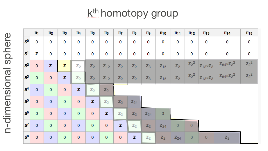
Let’s go through the theorems that fill in this table:

In the first row, S0 is the booleans, so these calculations follow from Hedberg’s theorem, which entails that the booleans are a set.
In the second row, S1 is the circle. Our calculation of this row consists of showing that the loop space of the circle (Ω(S1)) is Z: Applying truncation to both sides shows that π1(S1) is Z. Moreover, because the higher homotopy groups of a type are constructed from the loop space of that type, we get that that the higher homotopy groups of the circle are the same as the higher homotopy groups of Z, and therefore trivial, again because Z is a set.
We have a few different proofs that Ω(S1) is Z. The first (by Mike Shulman), follows a standard homotopy-theoretic argument, showing that the total space of the universal cover of the circle is contractible. Another (by Guillaume Brunerie) shortens the original proof significantly, by factoring some of the reasoning out into a flattening lemma about total spaces of fibrations defined by recursion on higher inductives. Another proof (by Dan Licata) avoids calculating the total space of the cover, instead relying on calculations using the definition of the cover by circle recursion. The template introduced in this proof is now known as the encode-decode method.
The all-0 diagonals (the colored diagonals below the πn(Sn) diagonal) state that πk(Sn) is trivial for k<n. We have a few different proofs of this now. In fact, we have two definitions of the n-sphere (which should coincide, but we haven’t proved this yet). The first is by induction on n: S1 is the circle, and the (n+1)-sphere is the suspension of the n-sphere. The second uses a fancy form of higher inductive types: First, we define the n-fold iterated loop space of a type, Ωn(A), by induction on n. Then, we define the n-sphere to be a higher inductive type with one point and one element of Ωn. The circle is generated by a point and a single 1-dimensional loop; the 2-sphere by a single point and a single 2-dimensional loop, and so on. This form of higher-inductive type is a bit unusual (and has not been formally studied): for each instantiation of n, the n-loop constructor is an element of a path type of Sn, but the level of iteration of the path type depends on n, and when n is a variable, Ωn is not syntactically a path type. However, the fact that the homotopy groups have come out right so far provides some indication that this is a sensible notion.
The first proof of πk<n(Sn) (by Guillaume Brunerie), for the suspension definition of the spheres, uses a connectedness argument. The second (by Dan Licata), for the iterated-loop-space definition, uses the encode-decode method. A third (by Dan Licata) uses a connectedness argument for π1 and then uses the Freudenthal suspension theorem (see below) to induct up.
For a long time after the first proof of π1(S1) in spring 2011, we were stuck on calculating any non-trivial higher homotopy groups. The thing that really broke the dam open on these was a proof of π2(S2) (by Guillaume Brunerie), which goes by way of proving that the total space of the Hopf fibration (as constructed by Peter Lumsdaine) is S3. This gives π2(S2), and also implies that πk(S2) = πk(S3), for k>=3. Because we have now calculated π3(S3) (see below), this gives π3(S2) = Z. Because we have now calculated most of π4(S3) (see below; the “most of” disclaimer is why these squares are shaded white in the table), this gives most of π4(S2). The grey shading on the remainder of the S2/S3 rows indicates that while we have not calculated any of these groups, we know that the two rows are equal.
The calculation of the total space of the Hopf fibration has proved difficult to formalize, because a key lemma requires some significant path algebra. However, only a couple of days after the first proof of π2(S2), we had a computer-checked one (by Dan Licata), using the encode-decode method, with the Hopf fibration playing the same role that the universal cover plays for S1. This proof bypasses showing that the total space of the Hopf fibration is S3, so it doesn’t give all the nice corollaries mentioned above. But it also illustrates that type theory can lead to shorter and more “beta-reduced” proofs of these theorems. This proof was for the iterated-loop-space definition of S2, but we eventually developed an encode-decode proof (also by Dan Licata) for the suspension definition.
Next, we have the πn(Sn) = Z diagonal. The proof is by induction on n, using π1(S1) in the base case, and proving that πn(Sn) = πn+1(Sn+1) in the inductive step. We have a couple of proofs of this. The first (by Dan Licata and Guillaume Brunerie) is a generalization of the encode-decode proof of π2(S2). It took about two weeks to develop and formalize the proof, much of which is a library exploring the type theory of iterated loop spaces. The second proof, for the suspension definition of the spheres, uses the Freudenthal suspension theorem.
The Freudenthal suspension theorem gives the connectedness of the path constructor for suspensions. It implies that all entries in the colored diagonals in the above chart are the same. Therefore, it suffices to compute one entry in each diagonal. We have done this for πk<n(Sn), for πn(Sn), and for πn+1(Sn) (shaded white). The remaining diagonals are shaded grey because we have proved that all entries are the same, but we haven’t calculated any individual entry.
The proof of the Freudenthal suspension theorem (by Peter Lumsdaine; formalized by Dan Licata) is an interesting combination of the encode-decode method used in πn(Sn) with the homotopy-theoretic notion of connectedness of maps and spaces. Indeed, the tower of results going from π2(S2) to πn(Sn) to Freudenthal really illustrates the promise of the interaction between homotopy theory and type theory: we started with a more homotopy-theoretic proof of π2(S2), which led to a more type-theoretic proof of π2(S2) (using the encode-decode method), which led to a more type-theoretic proof of πn(Sn), which led to a proof of the Freudenthal suspension theorem that combines these type-theoretic aspects with some additional homotopy-theoretic ideas about connectedness.
In the πn+1(Sn) = Z2 diagonal, we have a proof (by Guillaume Brunerie) that there exists a k such that π4(S3) = Zk, using the James construction. This diagonal is shaded white because this isn’t quite the classical result: we should also check that k is 2. However, this proof illustrates the promise of a computational interpretation of homotopy type theory: the proof is constructive, so to check that k is indeed 2, all we would need to do is run the program!

In addition to homotopy groups of spheres, we have proved the following theorems:

The Freudenthal suspension theorem gives information about spaces other than spheres. For example, we have a construction (by Dan Licata) of Eilenberg-Mac Lane spaces K(G,n), which are a basic building block that can be used to construct spaces up to homotopy equivalence. For an abelian group G, K(G,n) is a space whose nth homotopy group is G, and whose other homotopy groups are trivial; for example, K(Z,n) is equivalent to the n-truncation of the n-sphere. We first construct K(G,1), and then construct K(G,n) by suspending K(G,1) and truncating. The proof that it has the right homotopy groups uses the Freudenthal suspension theorem, generalizing the proof from Freudenthal that πn(Sn) = Z.
The Freudenthal suspension theorem gives the connectivity of the path constructor of a suspension. A generalization of suspensions is the notion of a pushout, and the generalization of Freudenthal to pushouts is the Blakers-Massey theorem. We have a proof of Blakers-Massey (by Peter Lumsdaine, Eric Finster, and Dan Licata; formalized by Favonia). We have also translated this proof to the language of ∞-topoi, which proves the result in a more general setting than was previously known.
van Kampen’s theorem characterizes the fundamental group of a pushout. We have a proof (by Mike Shulman; formalized by Favonia) using the encode-decode method.
To calculate π1(S1), we used the universal cover of the circle. This is an instance of a general notion of covering spaces, and the fact that covering spaces of a space correspond to actions by its fundamental group. Favonia formulated and formalized the theory of covering spaces.

You can find out more about these results in the following places:

Finally, there is a lot of low-hanging fruit left to pick! If you are interested in getting involved, leave a comment, or send an email to someone mentioned above (or to the HomotopyTypeTheory google group).

Universe n is not an n-Type

Joint work with Christian Sattler

Some time ago, at the UF Program in Princeton, I presented a proof that Universe n is not an n-type. We have now formalized that proof in Agda and want to present it here.

One of the most basic consequences of the univalence axiom is that the universe of types is not a set, i.e. does not have unique identity proofs. It is plausible to expect that the next universe $U_1$ is not a groupoid, i.e. its path-spaces are not sets, but a proof of that is already surprinsingly difficult.

We prove the generalized statement, namely that $U_n$ is not an n-type. At the same time, our construction yields, for a given $n$ , a type that is an $(n+1)$ -type but not an n-type. This answers one of the questions asked at the UF Program. The proof works in basic MLTT with $\Sigma$ -, $\Pi$ – and identity types as well as a sequence of universes. We need the uivalence axiom, but no other “HoTT-features”.

We also have a pdf version of the proof.

Covering Spaces

Covering spaces are one of the important topics in classical homotopy theory, and this post summarizes what we have done in HoTT. We have formulated the covering spaces and (re)proved the classification theorem based on (right) $\pi_1(X)$ -sets, i.e., sets equipped with (right) group actions of the fundamental group $\pi_1(X)$ . I will explain the definition and why we need some constancy factorization trick in the proof.

Definition

So, what are covering spaces in HoTT? The core ingredient of covering spaces is a fibration, which is easy in HoTT, because every function or dependent type in HoTT can be viewed as a fibration (up to homotopy). The only problem is the possible higher structures accidentally packed into the space (which are usually handled separately in classical homotopy theory). To address this, we have another condition that each fiber is a set. These two conditions together match the classical definition. More precisely, given a base space $X$ , a covering is a mapping $f$ from $X$ to some universe (or, a type family indexed by $X$ ) where for each $x \in X$ we know $f(x)$ is a set.

One can also formulate coverings as mappings instead of type families. I personally prefer the latter because they seem easier to work with in type theory. Note that we did not assert that the base space $X$ is path-connected or pointed, which are required by interesting theorems (ex: the classification theorem) but not by the definition.

Classification Theorem

The classification theorem says there is an isomorphism between $\pi(X,x_0)$ -set and covering spaces. Here we assume $X$ is path-connected and pointed (based) at $x_0 \in X$ .

The direction from covering spaces to $\pi(X,x_0)$ -sets is easier, since the set can simply be the fiber over the point $x_0$ , and the group action can be defined as transporting along an element in the homotopy group. The other direction is more challenging, requiring an explicit construction of the covering space from the given $\pi(X,x_0)$ -set. Naturally, the fiber over $x_0$ should be the underlying set, but what about other fibers? For arbitrary point $x$ in $X$ , due to the connectedness of the base space $X$ , there exists a (truncated) path from $x_0$ to $x$ , which can be used to transport everything in the fiber over $x_0$ to the fiber over $x$ . However, unless the homotopy group is trivial, one needs to identify multiple copies produced by different paths. We simply threw in gluing 1-cells and then made each fiber a set.

The above higher inductive type, which is called ribbon in the library, goes as follows: It is parametrized by the $\pi(X,x_0)$ -set, the underlying set $Y$ , the group action $\bullet$ , and the point $x$ in focus. The trace constructor “copies” everything from the fiber over $x_0$ to the fiber over $x$ along some path in the base type, and the paste constructor glues multiple copies made by different paths.

data ribbon (Y : Set) (∙ : Action Y) (x : X) : Set where
  trace : Y → Truncated 0 (x₀ = x) → ribbon x
  paste : (y : Y) → (loop : Truncated 0 (x₀ = x₀))
        → (p : Truncated 0 (x₀ = x))
        → trace (y ∙ loop) p ≡ trace y (loop ∘ p)

The most interesting part is to show that creating ribbons is left inverse to constructing $G$ -sets as mentioned in the beginning of the section. It suffices to show that ribbons indeed form the original covering space, which is, by functional extensionality, equivalent to demonstrating that they are fiberwise equivalent. The trouble is that, for a point $x \in X$ and a point $y$ in the fiber of the input covering over $x$ , one needs a path $x_0 = x$ to even make one point in the ribbon; while we can get a $(-1)$ -truncated path out of the connectedness condition, the constructor requires a $0$ -truncated path.

The constancy comes to rescue! It can be shown that, if there is a function $f$ from $A$ to a set $B$ , and $f$ is constant, then $f$ factors through $|A|$ with ideal computational behaviors. In our case, different points generated by different paths will be glued together by the paste constructor and moreover each fiber is a set. Therefore we can apply this lemma to establish the fiberwise equivalence, and hence the theorem!

Remarks

We also proved that the homotopy group itself corresponds to the universal covering, where universality is defined as being simply-connected. The ribbon construction, as an explicit description for covering spaces, comes in handy. In addition, we calculated $\pi(S^1)$ (again) with the new library; however, even with aggressive Agda optimization, the complexity remains—one still needs to prove the contractibility of some covering of $S^1$ for universality. Perhaps there are other better examples which can show the real power of this isomorphism?

The Agda code is currently available at http://hott.github.io/HoTT-Agda/Homotopy.Cover.HomotopyGroupSetIsomorphism.html but we are rebuilding the whole library. This link might not be valid after the migration.

Homotopy Theory in Homotopy Type Theory: Introduction

Many of us working on homotopy type theory believe that it will be a better framework for doing math, and in particular computer-checked math, than set theory or classical higher-order logic or non-univalent type theory. One reason we believe this is the “convenience factor” provided by univalence: it saves you from doing a lot of tedious proofs that constructions respect equality. When restricted to sets, univalence says that all constructions respect bijection, and this can be used to build algebraic structures in such a way that isomorphic structures are equal (e.g. equality of groups is group isomorphism), and therefore all constructions on structures automatically respect isomorphism. When restricted to 1-types, univalence can be used to define categories in such a way that equivalent categories are equal, and therefore all constructions are non-evil; moreover, these non-evil categories can coexist with a notion of strict category, which can be used when finer distinctions are necessary. In these applications, one defines the mathematical entities in question in a more or less traditional manner (a group is a type equipped with a multiplication operation, etc.), and univalence provides some theorems for free about constructions on these entities.

However, another reason we believe that HoTT will be a better framework, at least for certain kinds of math, is that it provides a direct way of working with something called ∞-groupoids. ∞-groupoidsare an infinite-dimensional generalization of the categorical notion of a groupoid (which is a category where every morphism is invertible). Where a groupoid has just objects and morphisms, ∞-groupoids have objects, morphisms, morphisms between morphisms (2-morphisms), … all the way up. ∞-groupoids are a complex structure: Morphisms at each level have identity, composition, and inverse operations, which are weak in the sense that they satisfy the groupoid laws (associativity of composition, identity is a unit for composition, inverses cancel) only up to the next level morphisms. Because of weakness, it is quite difficult to describe all of the operations/properties of morphisms. For example, because associativity of composition of morphisms (p o (q o r) = (p o q) o r) is itself a higher-dimensional morphism, one needs an additional operation relating different proofs of associativity; for example, the different ways to reassociate p o (q o (r o s)) into ((p o q) o r) o s give rise to Mac Lane’s pentagon. Weakness also creates non-trivial interactions between levels, such as the middle-four interchange law.

Now, the really cool thing about using HoTT to work with ∞-groupoids is that you don’t start by defining “an ∞-groupoid is…“like one would in any other framework—which is fortunate, because describing the structure of an ∞-groupoid in something like set theory is notoriously difficult, because of all the structure mentioned above.Instead, you exploit the fact that every type in type theory is an ∞-groupoid, with the structure of morphisms, 2-morphism, 3-morphisms, … given by the identity type (“propositional equality”).

Eventually, we hope to show that you can do a lot of math in an elegant way by working directly with ∞-groupoids, but for now, the area that we have developed the most is homotopy theory. I startedwritingan update on our recent progress doing homotopy theory in type theory, and realized that we didn’t have a post on the blog explaining the basics. So this post will tell the basic story: what is homotopy theory? How do we do it in type theory? And later I’ll post an update with what we’ve been up to recently.

Classical Homotopy Theory

Topology is the study of spaces up to continuous deformation. Algebraic topology is the use of tools from abstract algebra, like group theory, to tell whether two spaces are the same. As a first cut, we can say that two spaces are “the same” when there is an isomorphism between them (continuous maps back and forth that compose to the identity), though we will refine this later. For example, one basic construction in algebraic topology is the fundamental group of a space: Given a space X and a point x0 in it, one can (almost—see below) make a group whose elements are loops at x0 (paths from x0 to x0), with the group operations given by the identity path (standing still), path concatenation, and path reversal. Isomorphic spaces have the same fundamental group, so fundamental group can be used to tell two spaces apart: if X and Y have different fundamental groups, they are not isomorphic. Thus, the fundamental group is an algebraic invariant that provides global information about a space, which complements the local information provided by notions like continuity. For example, the torus (donut) locally looks like the sphere, but has a global difference: it has a hole in it. One way to see this is to observe that the fundamental group of the sphere is trivial, but the fundamental group of the torus is not.

To explain why this is so, we need to be a little more precise about what the fundamental group is. Consider a space X with a path p from x to y. Then there is an inverse path !p from y to x. Concatenating p with !p (written !p o p) gives a path from x to x, which should be the same as the identity path (witnessing one of the inverse cancellation laws of a groupoid). However, in topology, a path p in X is represented as a continuous map from the interval [0,1] into X, where p(0) = x and p(1) = y—think of the interval as “time” and p as giving the point on the path at each moment in time. Under this definition, !p o p (which walks from x to y, and then back along the same route, as time goes from 0 to 1) is not literally the same as the identity path (which stays still at x at all times). So loops don’t actually form a group!

The way to fix this is to consider the notion of homotopy between paths. Because !p o p walks out and back along the same route, you know that you can continuously shrink !p o p down to the identity path—it won’t, for example, get snagged around a hole in the space. Formally, a homotopy between functions f, g : X -> Y is a continuous map h : [0,1] * X -> Y such that h(0,x) = f(x) and h(1,x) = g(x). In the specific case of paths p and q, which, remember, are represented by maps [0,1] -> X, a homotopy is a continuous map h(t,x) : [0,1] x [0,1] -> X, such that h(0,x) = p(x) and h(1,x) = q(x). That is, it’s the image in X of a square, which fills in the space between p and q. Homotopy is an equivalence relation, and operations like concatenation, inverses, etc. respect it. Moreover, the homotopy-equivalence-classes of loops in X at x0 (where two loops p and q are equated when there is a based homotopy between them, which is a homotopy h as above that additionally satisfies h(t,0) = h(t,1) = x0 for all t) do form a group: while !p o p is not equal to the identity, it is homotopic to it! So, we can fix up the above definition of the fundamental group of a space by defining it to be the group of loops modulo homotopy.

Returning to the example, we can see that the sphere is different than the torus because the fundamental group of the sphere is trivial (the one-element group), but the fundamental group of the torus is not. The intuition is that every loop on the sphere is homotopic to the identity, because its inside is filled in. In contrast, a loop on the torus that goes around the donut’s hole is not homotopic to the identity, so there are non-trivial loops.

It turns out that the fundamental group, which is written π1(X,x0), is the first in a series of homotopy groups that provide additional information about a space. Fix a point x0 in X, and consider the constant path id at x0. Then the homotopies between id and itself form a group (when you quotient them by homotopy), which tells you something about the two-dimensional structure of the space. Then π3(X,x0) is the group of homotopies between homotopies, and so on. One of the basic questions that algebraic topologists consider is calculating the homotopy groups of a space X, which means giving a group isomorphism between πk(X) and some more direct description of a group (e.g., by a multiplication table or presentation). Somewhat surprisingly, this is a very difficult question, even for spaces as simple as the spheres. Here is a chart that lists the low-dimensional homotopy groups of the low-dimensional spheres (0 is the trivial group, Z is the integers, Zk is the the finite group Z mod k):

There are some patterns, but there is no general formula, and many homotopy groups of spheres are currently unknown. Homotopy groups are just one of the algebraic invariants that people study; some others are the homology groups and cohomology groups, which are sometimes easier to calculate.

An interesting fact is that, while we started off by trying to classify spaces up to isomorphism, most of these algebraic tools in fact classify spaces up to something called homotopy equivalence. Two spaces X and Y are homotopy equivalent iff there are maps f : X -> Y and g : Y -> X such that there is a homotopy between f o g and the identity function (and similarly for g o f). This gives you a little wiggle room to “correct” maps that don’t exactly compose to the identity, but only miss by space that can be filled in. Isomorphic spaces are homotopy equivalent, but not nice versa: for example, the disk is not isomorphic to the point, but it is homotopy equivalent to it. The vast majority of the constructions one considers (homotopy groups, homology and cohomology groups, etc.) are homotopy-invariant, in the sense that they respect homotopy equivalence. For example, two homotopy-equivalent spaces have the same fundamental groups, essentially because the fundamental group was defined to be paths modulo homotopy. Thus, these invariants are really properties of the homotopy-equivalence-classes of spaces, which are called homotopy types. If you’re interested in showing disequalities of spaces, this still has bearing on the original problem of classifying spaces up to isomorphism: if two spaces have different fundamental groups, then they are not homotopy equivalent, and therefore not isomorphic. One reason the fact that all of these notions are homotopy-invariant is important is that it enables a big generalization of classical homotopy theory.

Homotopy Theory of ∞-groupoids

Topological spaces are an instance of the notion of ∞-groupoid described above: every topological space X has a fundamental ∞-groupoid whose k-morphisms are the k-dimensional paths in X. The weakness of the ∞-groupoid (the fact that the groupoid laws hold only up to higher-dimensional morphisms) corresponds directly to the fact that paths only form a group up to homotopy, because the k+1-paths are the homotopies between the k-paths.

Moreover, the view of a space as an ∞-groupoid preserves enough structure to do homotopy theory (calculate homotopy/homology/cohomology groups, etc). Formally, the fundamental ∞-groupoid construction is adjoint to the geometric realization of an ∞-groupoid as a space, and this adjunction preserves homotopy theory (this is called the homotopy hypothesis/theorem, because whether it is a hypothesis or theorem depends on how you define ∞-groupoid). For example, you can easily define the fundamental group of an ∞-groupoid, and if you calculate the fundamental group of the fundamental ∞-groupoid of a space, that will agree with the classical definition of fundamental group. For the type theorists in the crowd: ∞-groupoids are an interface that topological spaces implement, and one can do homotopy theory using only the operations in the interface. The only problem is that this interface is fairly difficult to work with…

Homotopy Theory in Type Theory

Which is where type theory comes in! Type theory is a formal calculus of ∞-groupoids. Because you can do homotopy theory through the abstraction of ∞-groupoids, you can do homotopy theory in type theory. One might call this synthetic homotopy theory, by analogy with synthetic geometry, which is geometry in the style of Euclid: you start from some basic constructions (a line connecting any two points) and axioms (all right angles are equal), and deduce consequences from them logically. Here, the basic constructions/axioms are the operations on ∞-groupoids and maps between them (∞-functors), as presented by the identity type Id M N in dependent type theory. We will often refer to features of type theory by topological-sounding names (for example, thinking of p : Id M N as a “path” from M to N, or even writing Path M N for the identity type), but it’s important to keep in mind that we can only talk about these things through the abstraction of an ∞-groupoid.

There are few really nice advantages of doing synthetic homotopy theory in type theory. First, you can use proof assistants like Agda and Coq to check your proofs. Second, we’re starting to see examples where working in type theory is suggesting new ways of doing proofs. Third, it seems likely that we will be able to interpret type theory in a wide variety of other categories that “look like” ∞-groupoids, and, if so, proving a result in type theory will show that it holds in these settings as well. It remains to be seen how much homotopy theory we can do synthetically, but there are already some positive indication, which I’ll discuss in a following post.

For now, I’d like to review the basic ingredients of doing synthetic homotopy theory in type theory, with some links to reading material:

Higher inductive types. To do some homotopy theory, we need some basic spaces (the circle, the sphere, the torus) and constructions for making new spaces (suspensions, gluing on cells, …). These are defined using higher inductive types, which are inductive types specified by both point and path constructors.

For example, the circle is inductively generated by base:S1 and loop:Path base base—an inductive type with one point and one non-trivial loop. This inductive type describes the free ∞-groupoid with one object and one 1-morphism. The elimination rule for the circle, circle induction, expresses freeness: a map f : S1 -> X, from the circle into some type X is specified by giving a point and a loop in X (the image of the generators), and the general rules for the identity type ensure that f preserves the groupoid structure (e.g. it commutes with composition).

Higher inductive types are very general, and allow one to build spaces that are specified by a CW complex, using suspensions, pushouts, etc. This gives a logical/synthetic view of these spaces, where they are constructed as the free ∞-groupoid on some generators, and can be reasoned about using induction.

Homotopy groups. Havingdefined some spaces, we’d like to start calculating some algebraic invariants of them. The homotopy groups have an extremely natural definition in the setting of ∞-groupoids/type theory. The fundamental group of X at x0 is (to a first approximation—see below) just the identity type Id{X} x0 x0, or the morphisms of the ∞-groupoid; π2(X,x0) is just the identity type Id{Id{X} x0 x0} refl refl, or the 2-morphisms, etc. So, calculating a homotopy group is just giving a bijection between an identity type and some other type, and proving that this bijection preserves the group structure. For example, calculating the fundamental group of the circle consists of giving a bijection between Id{S1} base base and Int that sends composition of paths to addition.

The reason this problem is interesting is that the (higher) inductive definition of a type X presents X as a free ∞-groupoid, and this presentation determines but does not explicitly describe the higher identity types of X. The identity types are populated by both the generators (loop, for the circle), and all of the groupoid operations (identity, composition, inverses, …). As the above table for spheres shows, in higher dimensions the ∞-groupoid operations create quite a complex structure. Thus, the higher-inductive presentation of a space allows you to pose the question “what does the identity type of X really turn out to be?”, though it can take some significant math to answer it. This is a higher-dimensional generalization of a familiar fact in type theory: even for ordinary inductive types like natural numbers or booleans, it takes a bit of work to prove that true is different than false—characterizing the identity type at bool is a theorem, not part of the definition.

The one detail that I glossed over above is that the (iterated) identity type really gives what is called the path space of a space, which is not just the set of k-dimensional path, but a whole space of them, with their higher homotopies. To extract the set of paths-modulo-homotopy, we can use something called truncation.

N-types and truncations. One of Voevodsky’s early observations was that it is possible to define a homotopy-theoretic notion called being an n-type in type theory. He called these “types of h-level n”, and started counting at 0, but many of us now call them type levels or truncation levels and use the traditional homotopy-theoretic numbering, which starts at -2. A -2-type (“contractible”) is equivalent to the unit type. A -1-type (“hprop”) is proof-irrelevant—any two elements are propositionally equal. A 0-type (“hset”) has uniqueness of identity proofs—any two propositional equalities between its elements are themselves equal. A 1-type is like a groupoid: it can have non-trivial morphisms, but all 2-morphisms are trivial. And so on. Categorically, n-types correspond to n-groupoids.

The predicate “X is an n-type” is part of a modality, which means that there is a corresponding operation of n-truncation that takes a type A and makes the best approximation of A as an n-type. n-truncation equates (“kills”) all morphisms of level higher than n in A. Truncations can be constructed using higher inductive types (see here and here) and are quite important to doing homotopy theory in type theory, because many theorems characterize some “approximation” of a space, where the approximation is constructed by truncation.

For example, the fundamental group of a space is defined to be the 0-truncation of the space of loops at x0, which produces the hset of paths modulo homotopy, killing the higher homotopies of the loop space.

Univalence. The univalence axiom plays an essential role in calculating homotopy groups (this is a formal claim: without univalence, type theory is compatible with an interpretation where all paths, including e.g. the loop on the circle, are the identity). You can see this in action in the calculation of the the fundamental group of the circle: the map from Id{S1} base base to Z is defined by mapping a path on the circle to an isomorphism on Z, so that, for example, loop o !loop is sent to successor o predecessor, and then applying the isomorphism to 0. Univalence allows paths in the universe to have computational content, and this is used to extract information from paths in higher inductive types.

Homotopy-theoretic and type-theoretic methods. One of the cool things we’ve found is that there are different ways of doing proofs in homotopy type theory. Some proofs use techniques that are familiar from traditional homotopy theory, whereas others are more type-theoretic, and consist mainly of calculations with the ∞-groupoid structure. For example, Mike Shulman’s original calculation of the the fundamental group of the circle is more homotopy-theoretic, while mine is more type-theoretic. You can read more about the difference between the two in this paper.

Those are the basic tools. In the next post, I’ll give an overview of the current status of homotopy theory in HoTT.

Running Spheres in Agda, Part II

(Sorry for the long delay after the Part I of this post.)

This post will summarize my work on defining spheres in arbitrary finite dimensions (Sⁿ) in Agda. I am going to use the tools for higher-order paths (discussed in Part I) to build up everything for spheres. There are many ways to define a sphere and I will stick with the “one 0-cell and one n-cell” definition in this post. One important feature is that I have achieved full compatibility with previous ad-hoc definitions for specific dimensions (ex: S²) except for one small caveat mentioned below. That is, this is a drop-in replacement for spheres ever defined for any fixed dimension in 95% cases. The code is available at this place.

Why is this Difficult?

The most difficult thing is the computation rule for loops. It is tricky to get the types right, and is even trickier to derive the non-dependent rule from the dependent one. Intuitively, this rule says “if I plugged in some data for the loop in the eliminator, then applying this instantiated eliminator to the original loop will recover that data I plugged in”. This looks fine, except that the types do not (immediately) match in Agda. We need to find a way to talk about the types of the plugged-in data without mentioning the eliminator itself. The reason is that, when we are declaring the eliminator, the type cannot mention the name of the eliminator itself in Agda (at least in my understanding). However, when you are applying this instantiated eliminator to the original loop, the result will have the eliminator in the type, and in general it is not definitonally equal to the type we used in the declaration of the eliminator. This mismatch becomes a serious problem for arbitrary finite dimensions.

S¹ in Agda luckily avoids this problem because of the definitional equality for 0-cells (base points) and its finite dimension. However, it can still illustrate the problem if we pretend that there was only evidential equality for 0-cells. Let’s look at the type of eliminator in Agda:

S¹-elim : ∀ {ℓ} (P : S¹ → Set ℓ) (pbase : P base)
          → subst P loop¹ pbase ≡ pbase
          → (x : S¹) → P x

pbase is the data for the base point and subst P loop¹ pbase ≡ pbase is the type of the data for the loop. The holy grail of the definition of S¹ is then the following equivalence:

cong[dep] P (S¹-elim P pbase ploop) loop¹ ≡ ploop

where cong[dep] is the dependent map on paths (which is named map or apd in different HoTT libraries). This equivalence means that we can recover the plugged-in data by applying the eliminator to the original loop. The trouble is that this is ill-typed unless we have some definitional equality. The type of the left-hand side is actually

subst P loop¹ ((S¹-elim pbase ploop) base) ≡ ((S¹-elim pbase ploop) base)

while the right-hand side is of type

subst P loop¹ pbase ≡ pbase

How do we know that the eliminator applied to the base point is indeed the data for the base point? This is why the Coq library required (thanks to a recent patch) requires (or at least “required”—I am not aware of the possible recent development) some extra work to bridge the gap in types. When we are defining spheres for a particular dimension, the type checker (equivalently) kindly expands the expressions down to eliminators applied to the base points. (This is of course not what a type checker in Coq/Agda really does.) The way we use Agda will establish the definitional equivalence between this application and the data for the base point, and so the type checker is satisfied.

Nonetheless, Agda cannot expand the expressions for us if we are talking about spheres in arbitrary finite dimensions. It requires an induction on the dimension to show that two things are equivalent, which is beyond the ability of the current type checker. We need to prove the equivalence by ourselves.

In the following paragraphs I will describe how I have proved necessary lemmas to bridge the gap. Moreover the lemmas appearing in types will “go away” if you plug in any finite number for the dimension. This makes the library a drop-in replacement of previously defined sphere in most cases. The only missing feature is that, while non-dependent elimination rules are derived from the dependent ones, the non-dependent computation rules for loops are not. A 100% drop-in replacement should have all non-dependent rules derived from dependent counterparts.

Technical Discussion

Towers of Loops

Let’s set up the n-cell in spheres so that we can talk about computation rules. They are basically higher-order loops, that is, towers of loops:

S-endpoints⇑ 0 base = lift tt
S-endpoints⇑ (suc n) base = (S-endpoints⇑ n base , S-loop⇑ n base , S-loop⇑ n base) 

S-loop⇑ 0 base = base
S-loop⇑ (suc n) base = refl (S-loop⇑ n base)

whose data are filled by two mutually recursive functions where n is the dimension. We can then fake the loop (n-cell) constructor by a postulation in Agda:

postulate
  loopⁿ : ∀ n → Path⇑ n (S-endpoints⇑ n (baseⁿ n))

The elimination rule for spheres is shown below, where S-endpoints[dep]⇑ is the dependent loop tower parametrized by the mapped base point. This is probably not so surprising if you are familiar with S¹ in Agda. The scary type in the middle means “the path built from the dependent form of the loop and the data for the base point”. For S¹ this is simply subst P loop¹ pbase ≡ pbase. The last line establishes the definitional equality for the base point.

Sⁿ-elim : ∀ {ℓ} n (P : Sⁿ n → Set ℓ) (pbase : P (baseⁿ n))
          → Path[dep]⇑ n P (loopⁿ n) (S-endpoints[dep]⇑ n P (baseⁿ n) n P pbase)
          → ∀ x → P x
Sⁿ-elim n P pbase _ baseⁿ′ = pbase

Fix the Type Mismatch in Computation Rules

We already have computation rules for base points for free (by Dan’s trick). The remaining type mismatch mentioned above is due to lack of (definitional) communicativity between “building towers” and “applying functors” in Agda. That is, we want to show that building a tower of loops as above, and then mapping the whole tower to another space, is equivalent to mapping the base point to the target space first and then building up the tower right within that space. This is done by an induction on the dimension; we walk down the tower by repetitively applying the J rule.

Again (as in Part I), the way the tower is presented is important. It is difficult, if not impossible, to walk down the tower if the tower is upside down—that the outermost loop is the loop in the lowest dimension. My ordering (which exposes the path (or the loop here) in the highest dimension) makes this task easy. The particular induction here involves two mutually recursively defined functions to deal with different data in the tower. This is somewhat expected as we adopted mutually recursive functions to build towers as well.

One feature is that the usage of the J rule within this lemma is carefully arranged so that, in any given finite dimension, the proof will be definitionally equivalent to refl. This means that any previous code that depends on a sphere in some fixed dimension will not notice this artifact.

Non-dependent Rules

The final note is about the definition and derivibility of non-dependent rules.

For non-dependent elimination rules, we have to show that, a non-dependent tower is equivalent to a dependent tower with a “constant” type family. (Sorry but I am not sure about the accurate terminology here.) This can be achieved by the same technique—walking down the tower to the ground.

The type of the non-dependent computation rule has the same type mismatch issue, and can be solved by the technique mentioned above—but for non-dependent constructs this time.

On the other hand, the derivability of the non-dependent computation rule seems quite involved and so I have not finished it. Fortunately, I am not aware of any code that depends on the assumption that the non-dependent computation rule is derived from the dependent version.

Thanks to many people (Dan Licata, Bob Harper, etc) for helping me overcome my laziness.

On h-Propositional Reflection and Hedberg’s Theorem

Thorsten Altenkirch, Thierry Coquand, Martin Escardo, Nicolai Kraus

Overview

Hedberg’s theorem states that decidable equality of a type implies that the type is an h-set, meaning that it has unique equality proofs. We describe how the assumption can be weakened. Further, we discuss possible improvements if h-propositional reflection (“bracketing”/”squashing”) is available. Write X* for the h-propositional version of a type X. Then, it is fairly easy to prove that the following are logically equivalent (part of which Hedberg has done in his original work):

X is h-separated, i.e. ∀ x y → (x ≡ y)* → x ≡ y
X has a constant endofunction on the path spaces, i.e. we have a function f: (x y: X) → x ≡ y → x ≡ y and a proof that f x y is constant for all x and y
X is an h-set, i.e. ∀ x y: X → ∀ p q: x ≡ y → p ≡ q

We then state the three properties for arbitrary types instead of path spaces. For a type A, the first two statements become

A is h-stable, i.e. A* → A
A has a constant endofunction, i.e. f: A → A and a proof of ∀ a b → fa ≡ fb

Clearly, the first statement is at least as strong as the second, but somewhat surprisingly, the second also implies the first. The proof of this fact is non-trivial.
In this blog post, we mainly talk about the mentioned results and try to provide some intuition. This is actually only a small part of our work. Many additional discussions, together with formalized proofs, can be found in this Agda file. Thanks to Martin, it is a very readable presentation of our work.

Generalizations of Hedberg’s Theorem

Having this proof of Hedberg’s Theorem in mind, the essence of the theorem can be read as:

(i) If we can construct an equality proof whenever we have h-propositional evidence that there should be one, then the type is an h-set.

Here, we call a type h-propositional (or an h-proposition) if all its elements are equal. Intuitively, decidable equality is much stronger than the property mentioned above: If we have a function dec that decides equality and x, y are two terms (or points), we do not even require evidence to get a proof that they are equal. Instead, we can just apply dec to get such a proof or the information that none exists.

It is therefore not surprising that Hedberg’s theorem can be strengthened by weakening the assumption. For example, a proof of ¬¬ x ≡ y could serve as evidence that x, y are equal; and indeed, if we know that a type is separated, i.e. that we have ∀ x y → (¬¬ x ≡ y) → x ≡ y, then the type is an h-set. This requires a weak form of extensionality (to show that ¬¬ x ≡ y is an h-proposition) and the controverse is not true.

In the presence of h-propositional reflection, we can do much better. We define h-propositional reflection as an operation _* from types to h-propositions (viewed as a subsets of types) that is left adjoint to the embedding, i.e. we have a universal property. These are Awodey’s and Bauer’s bracket types: The idea is that, given a type X, the type X* corresponds to the statement that there exists an inhabitant of X (we say that X is h-inhabited if we have p: X*). We always have the map η: X → X*. From X*, we do usually not get X, but if we could prove an h-proposition from X, then X* is sufficient. It is natural to consider h-propositional reflection in our context, because the informal notion “h-propositional evidence, that a type is inhabited” can now directly be translated. We call a type satisfying (i) in this sense h-separated: h-separated X = ∀ x y → (x ≡ y)* → x ≡ y.

In Hedberg’s original proof, it is shown that a constant parametric endofunction on the path spaces is enough to ensure that a type is an h-set. For a function f, we define that f is constant by constant f = ∀ x y → fx ≡ fy. As already mentioned above, it is fairly straightforward to show:

Theorem. For a type X, the following properties are logically equivalent:

X is h-separated, i.e. ∀ x y → (x ≡ y)* → x ≡ y

X has a constant endofunction on the path spaces, i.e. we have a function f: (x y: X) → x ≡ y → x ≡ y and a proof that f x y is constant for all x and y

X is an h-set, i.e. ∀ x y: X → ∀ p q: x ≡ y → p ≡ q

For this reason, we consider h-separated X → h-set X the natural strengthening of Hedberg’s theorem. The assumption is now the exact formalization of the condition in (i), the assumption is as weak as it can be (as it is necessary) and, in particular, it is immediately implied by Hedberg’s original assumption, namely the decidable equality property.

H-propositional Reflection and Constant Endofunctions

The list of equivalent statements above suggests that one could look at these statements for an arbitrary type A, not only for the path spaces. Of course, they do not need to be equivalent any more, but they become significantly simpler:

A is h-stable, i.e. A* → A
A has a constant endofunction, i.e. f: A → A and a proof of ∀ a b → fa ≡ fb
A is an h-proposition, i.e. ∀ a b: A → a ≡ b

For the third, it is pretty clear what this means and it is obviously strictly stronger than the first and the second. If A is h-stable, we get a constant endofunction by composing η: A → A* with A* → A. However, it is nontrivial whether a type with a constant endofunction is h-stable. Somewhat surprisingly, it is.

But let us first consider the question we get if we drop the condition that we are dealing with endofunctions. Say, we have f: X → Y and a proof c: constant f. Can we get a function X* → Y?
Consider the chaotic equivalence relation on X, which just identifies everything: x ~ y for all x and y, which is h-propositional (~: X → X → hProp with x ~ y = True for all x and y, if we want). According to the usual definition of a quotient, our constant map f can be lifted to X/~ → Y. So, what we asked can be formulated as: Does X* have the properties of X/~? If Y is an h-set, this lifting exists (Voevodsky makes use of this fact in his definition of quotients), but otherwise, our definition of constant is too naïve, as it involves no coherence conditions at all. If we know that Y has h-level n, we can try to formulate a stronger version of constant that solves this issue. This could be discussed at another opportunity. With the naïve definition of constant, we would have to make a non-canonical choice in X, but f only induces an “asymmetry” in Y.

Let us get back to the case where f is a constant endofunction. We still do not have the coherence properties mentioned above, but the asymmetry of Y is now an asymmetry of X and, somewhat surprisingly, this is sufficient. We have the following theorem:

Theorem. A type X is h-stable (X* → X) iff it has a constant endofunction.

Note that the direction from right to left is easy. For the other direction, we need the following crucial lemma:

Fixpoint Lemma (N.K.). If f: X → X has a proof that it is constant, then the type of fixed points Σ(x:X) → x ≡ fx is h-propositional.

Let us write P for the type Σ(x:X) → x ≡ fx. A term of P is a term in X, together with the proof that it is a fixed point. With the lemma, we just have to observe that there is the obvious map X → P, namely λx → (fx , constant x fx) to get, by the universal property of *, a map X* → P. Composed with the projection map P → X, this gives us the required map showing that X is h-stable.

To prove the lemma, we need the following two observations. For both, we assume that X, Y are types and x,y: X terms. Further, we write p • q for trans p q, so that this typechecks if p: x ≡ y and q: y ≡ z. We use subst (weak version of J) and cong (to apply functions on proofs) in the usual sense.

Observation 1. Assume h, k: X → Y are two functions and t: x ≡ y as well as p: h(x) ≡ k(x) are paths. Then, subst t p is equal to (cong h t)⁻¹ • p • (cong k t).

This is immediate by applying the equality eliminator on (x,y,t). We will need this fact for a proof of type t : x ≡ x, but this required special case cannot be proved directly.

The second observation can be considered the key insight for the Fixpoint Lemma:

Observation 2. If f: X → Y is constant, then cong f maps any proof of x ≡ x to reflexivity.

It is not possible to prove this directly. Instead, we formulate the following generalization: If c: constant f is the proof that f is constant, then cong f maps any proof p: x ≡ y to (c x x)⁻¹ • (c x y). This is immediate by using induction (i.e. the J eliminator) on (x,y,p), and it has the above statement as a consequence.

Proof (of the Fixpoint Lemma). Assume we have f: X → X, c: constant f and (x,p), (x',p'): Σ (x: X) → x ≡ fx. We need to show that these pairs are equal. It is easy to prove x ≡ x' by composing the proofs p: x ≡ fx, constant x x': fx ≡ fx' and (p')⁻¹: fx' ≡ x'. We call this proof p'': x ≡ x'. Clearly, we have that (x, subst (p'')⁻¹ p') and (x',p') are equal now, just by the proof p'' for the first component, and the equality of the second components is immediate. We choose to write q for the proof subst (p'')⁻¹ p'. Now, we are in a slightly simpler situation: We need to show that (x,p) and (x,q) are equal.

If we prove that the first components are equal using some proof t: x ≡ x, then what we need for the second components is p ≡ subst t q. Clearly, using refl for t would not work.

By Observation 1, our goal is equivalent to proving p ≡ t⁻¹ • q • (cong f t).
Using Observation 2, this simplifies to p ≡ t⁻¹ • q. Let us therefore just choose t to be q • p⁻¹. This completes the proof of the Fixpoint Lemma and the Theorem. □

As mentioned, there is a bunch of possible further questions and considerations, but for now, we want to conclude with a question that we are not so sure about anymore: Is h-propositional reflection definable in MLTT (with extensionality)? With heavy use of the Fixpoint Lemma, we have come fairly close to such a definition. It should not be possible, but is there a proof of that fact?

On Heterogeneous Equality

(guest post by Jesse McKeown)

A short narative of a brief confusion, leading to yet-another-reason-to-think-about-univalence, after which the Author exposes his vaguer thinking to derision.

The Back-story

In the comments to Abstract Types with Isomorphic Types, Dan Licata mentioned O(bservational)TT, originating in works of McBride, with Altenkirche, McKinna… One of the initially-strange features therein is a so-called "heterogeneous equality" type, which from my very cursory reading I see has something to do with coercing along equivalences. Of course, this piqued my curiosity and a short-while later I happened upon this book about using coq as a practical program verification assistant, by way of this section of the chapter "Equality".

Continue reading →

All Modalities are HITs

Last Friday at IAS, Guillaume Brunerie presented a very nice proof that $\pi_k(S^n)=0$ for all $k <n$ . I hope he will write it up and blog about it himself; I want to talk instead about a question regarding modalities that was raised by his talk: is every modality a higher inductive type?

Continue reading →

Abstract Types with Isomorphic Types

Here’s a cute little example of programming in HoTT that I worked out for a recent talk.

Abstract Types

One of the main ideas used to structure large programs is abstract types. You give a specification for a component, and then you divide your program into two parts, the client and the implementation. In the latter, you implement the component with some concrete code that satisfies the specification. In the client, you use the functionality provided by the component—but, crucially, relying only on the spec, not the concrete implementation. This has lots of advantages: you can change each part independently; different people can work on each part simultaneously; when there’s a bug, you know who to blame….

Here’s a simple example, written in ML (I’ve included links to some lecture notes, in case there are people in the audience who would like more background on ML or on this kind of programming). The abstraction in question is that of a sequence, an ordered collection of values.

signature SEQ = 
sig
   type α seq 

   val empty  : α seq
   val single : α → α seq 
   val append : α seq → α seq → α seq 

   (* Behavior: map f < x1, ..., xn >  =  < f x1, ..., f xn > *)
   val map    : (α → β) → (α seq → β seq) 

   val reduce : (α → α → α) → α → α seq →  α 
end

The first line says that for any type α there is a type α seq. There are various ways of building sequences: you can make an empty one, a 1-element one, and you can concatenate two of them. And there are some ways of processing them: map applies a function to each element; reduce applies a binary operation to pairs of elements (e.g., reduce + 0 adds up all the elements in an int seq). I’ve given a behavioral spec for map only; in reality, you would say what the behavior of each operation is. A full sequence spec would have lots more operations, but hopefully you get the idea.

On the implementation side, you can do something simple, like implement sequences with lists:

structure ListSeq : SEQ = 
struct     
   type α seq = α list 
   val map = List.map
   ... 
end

or you might do something more complicated, like implementing sequences as some sort of tree or array for efficiency. Indeed, you can even give a parallel implementation of sequences

structure PSeq : SEQ =  ...

where map applies f to each element in parallel, reduce computes on a tree, and so on. Using this implementation of sequences, you can exploit the parallelism available in a multicore machine or in a computer cluster, while writing exactly the same clean functional code that you would have written in a sequential program. We teach this idea of data parallelism in our first-year FP course and second-year algorithms and data structures course at CMU.

Reasoning using Views

While abstract types get used all over ML and Haskell code, they are less common in dependently typed programming. Why? In simply-typed programming, it’s often good enough to have informal behavioral specs in comments (like (* map f < x1, ..., xn > = < f x1, ..., f xn > *)). But with dependent types, you usually need a formal behavioral spec for the component, in order to prove properties about the client code. One cheap (and common) solution is to avoid using abstract types, so that you can reason directly in terms of the implementation in the client code. But then you lose all the benefits of abstract types, and your reasoning is tied to a particular implementation! Moreover, it’s unclear how well this technique scales: as the implementation gets more sophisticated, the code often gets less useful for external reasoning in the client anyway (e.g., if you implement sequences with a balanced binary tree, your client code would need to talk about red-black invariants).

A better solution is to associate a concrete view type with the abstract type (Wadler and others have developed this technique for reasoning about and pattern matching on abstract types). One nice way to do this is to stipulate that (1) the abstract type is isomorphic to the view type and (2) all of the operations respect this isomorphism. In our running example, we could give a view of sequences as lists as follows (I’ll still use an ML-ish notation, but write ≃ for the identity type; Iso for a type of isomorphisms—functions back and forth that compose to the identity up to ≃; and show and hide for applying an isomorphism i in the forward and backward directions, respectively)):

signature SEQ' = 
sig
   type α seq 
   val i : Iso(α seq, α list )

   val empty  : α seq
   val empty_spec : show i empty ≃ []

   val single : α → α seq 
   val single_spec : ∀ (x) -> show i (single x) ≃ [x]

   val append : α seq → α seq → α seq 
   val append_spec : ∀ (s1 s2) -> show i (append s1 s2) ≃ (show i s1 @ show i s2)

   val map    : (α → β) → (α seq → β seq) 
   val map_spec : ∀ (s f) -> show i (map f s) ≃ (List.map f (show i s))

   val reduce : (α → α → α) → α → α seq →  α 
   val reduce_spec : ∀ (b u s) -> (reduce b u s) ≃ (List.reduce b u (show i s))

end

i is an isomorphism between the abstract type of sequences and a concrete view type, in this case lists. For each operation, we say how it is interacts with the view, essentially saying that each operation on sequences behaves like the corresponding operation on lists. E.g., map_spec says that the view of a map is the same as doing a List.map on the view—and, because List.map is defined inductively, this formalizes the above informal spec’s ....

These specs suffice to do proofs about the component, independent of the concrete implementation. The main idea is that properties can be derived from the corresponding properties for lists. For example, map fusion (functoriality)

map (g . f) ≃ map g . map f

is useful for optimizing a 2-pass algorithm into a one pass algorithm. To prove it, we can reason as follows (writing . for function composition and fromList/toList for hide/show i):

map (g . f)                                                           [by map_spec]
≃ fromList . List.map (g.f) . toList                                  [by fusion for List.map]
≃ fromList . List.map g . List.map f . toList                         [i is an isomorphism]
≃ fromList . List.map g . (toList . fromList) .  List.map f . toList   [associativity of .]
≃ (fromList . List.map g . toList) . (fromList . List.map f . toList) [by map_spec]
≃ map g . map f

Views in HoTT

There are a couple of reasons why the above kind of specification is annoying in current dependently typed programming languages. First of all, it’s pretty verbose, and in a boring sort of way: for each component of the signature, you need to give a spec, but these specs are all of the form X ≃ appropriately wrapped List.X. Second, while the specs fully characterize the operations up to the identity type, they have no definitional behavior—and in some cases, where the implementation has nice definitional behavior, the abstract version will be much less convenient to work with because of this.

We can easily solve the first problem in Homotopy Type Theory, as I will illustrate below. While I don’t have anything concrete to say about the second problem right now, part of the computational interpretation of univalence is going to involve developing better tools for pushing around propositional equalities, so, given this, hopefully the lack of definitional equalities won’t be as much of an issue.

Above, the code for the spec was linear in the size of the component. In Homotopy Type Theory, we can do it in one line! Define PSeq and ListSeq : SEQ as above, and then here’s the whole spec:

spec : PSeq ≃ ListSeq

Thinking of SEQ as a Σ-type, this spec entails everything that we said above:

there is an isomorphism between α PSeq.seq and α List.seq for each α.
This follows immediately from the “definition” of the identity type at each type: a path in Σ is a pair of paths; a path in Π is a family of paths; a path between types is an isomorphism (really, an equivalence, but because we’re talking about hsets I can ignore the coherence data).
each PSeq operation behaves like corresponding list operation.
First, the definition of path in a Σ-type says that the PSeq operations behave like the transport of the ListSeq operations along this isomorphism. Then, using the computation rules for transport, this simplifies to the specs given above: each PSeq operation behaves like the appropriate wrapping of the corresponding ListSeq with the view isomorphism.

In Coq or Agda, you can calculate this all out by hand, but because the proof is basically just computation, I expect that a proof assistant could easily expand the one-line spec into SEQ' programmatically. The point is that the process of annotating the signature with the behavioral spec is exactly an instance of the generic programming that is available in HoTT.

We could even go further and observe that the little derivations of facts like map fusion from the corresponding list properties can be abstracted away, but I won’t illustrate that there.

Non-isomorphic views?

One complaint that is typically levied against this kind of spec is that the implementation and the view are often not exactly isomorphic: there might only be functions back and forth, or a section/retraction. For example, if you implement sequences as binary trees, then there will be many associativities of a tree that are modelled by the same list: the concrete implementation might have a finer equivalence than what is desired for the abstract spec. Because we have quotient types available in HoTT, I would hope that we can handle this case, but this needs to be investigated on some examples.

Isomorphism implies equality

Thierry Coquand and I have proved that, for a large class of algebraic structures, isomorphism implies equality (assuming univalence).

A class of algebraic structures

Structures in this class consist of a type, some operations on this type, and propositional axioms that can refer to operations and other axioms.

N-ary functions are defined in the following way (using Agda notation):

_^_⟶_ : Set → ℕ → Set → Set
A ^ zero ⟶ B = B
A ^ suc n ⟶ B = A → (A ^ n ⟶ B)

The class of algebraic structures is then defined in two steps. In the first step codes for structures, Structure, are defined mutually with a decoding function, ⟦_⟧, using induction-recursion:

mutual

  infixl 5 _+operator_ _+axiom_

  data Structure : Set₁ where
    empty : Structure

    -- N-ary functions.
    _+operator_ : Structure → (n : ℕ) → Structure

    -- Arbitrary propositional axioms.
    _+axiom_ : (s : Structure)
               (P : Σ (∀ A → ⟦ s ⟧ A → Set) λ P →
                      ∀ A s → Propositional (P A s)) →
               Structure

  ⟦_⟧ : Structure → Set → Set₁
  ⟦ empty                 ⟧ A = ↑ _ ⊤
  ⟦ s +operator n         ⟧ A = ⟦ s ⟧ A × (A ^ n ⟶ A)
  ⟦ s +axiom (P , P-prop) ⟧ A = Σ (⟦ s ⟧ A) (P A)

Here Propositional B means that B is of h-level 1, and ↑ _ ⊤ stands for the unit type, lifted to Set₁.

In the second step the decoding function’s Set argument is instantiated:

⟪_⟫ : Structure → Set₁
⟪ s ⟫ = Σ Set ⟦ s ⟧

As a simple example of an algebraic structure in this class we can define semigroups (over sets). The definition uses function extensionality to prove that the axioms are propositional. Note that the first axiom states that the underlying type is a set. This assumption is used to prove that the other axiom is propositional:

semigroup :
  ({A : Set} {B : A → Set} → Extensionality A B) →
  Structure
semigroup ext =
  empty

  +axiom
    ( (λ A _ → Is-set A)
    , is-set-prop
    )

  +operator 2

  +axiom
    ( (λ { _ (_ , _∙_) →
           ∀ x y z → x ∙ (y ∙ z) ≡ (x ∙ y) ∙ z })
    , assoc-prop
    )

  where
  is-set-prop = …

  assoc-prop = λ { _ ((_ , A-set) , _) → … }

Semigroup :
  ({A : Set} {B : A → Set} → Extensionality A B) →
  Set₁
Semigroup ext = ⟪ semigroup ext ⟫

Isomorphisms

We can also define what it means for two structures to be isomorphic. The property of being an n-ary function morphism is defined in the following way:

Is-_-ary-morphism :
  (n : ℕ) {A B : Set} → (A ^ n ⟶ A) → (B ^ n ⟶ B) → (A → B) → Set
Is- zero  -ary-morphism f₁ f₂ m = m f₁ ≡ f₂
Is- suc n -ary-morphism f₁ f₂ m =
  ∀ x → Is- n -ary-morphism (f₁ x) (f₂ (m x)) m

This definition can be lifted to structures by ignoring the (propositional) axioms:

Is-structure-morphism :
  (s : Structure) →
  {A B : Set} → ⟦ s ⟧ A → ⟦ s ⟧ B →
  (A → B) → Set
Is-structure-morphism empty           _          _          m = ⊤
Is-structure-morphism (s +axiom _)    (s₁ , _)   (s₂ , _)   m =
  Is-structure-morphism s s₁ s₂ m
Is-structure-morphism (s +operator n) (s₁ , op₁) (s₂ , op₂) m =
  Is-structure-morphism s s₁ s₂ m × Is- n -ary-morphism op₁ op₂ m

Two “top-level” structures are then defined to be isomorphic if there is a homomorphic bijection between the corresponding Sets:

Isomorphism : (s : Structure) → ⟪ s ⟫ → ⟪ s ⟫ → Set
Isomorphism s (A , s₁) (B , s₂) =
  Σ (A ↔ B) λ m → Is-structure-morphism s s₁ s₂ (_↔_.to m)

Here m : A ↔ B means that m is a bijection from A to B, and _↔_.to m is the corresponding function of type A → B.

The result

Finally we can state the main result. Isomorphic structures are equal, assuming univalence:

Univalence-axiom′ (Set ²/≡) Set →
Univalence-axiom lzero →
(s : Structure) (s₁ s₂ : ⟪ s ⟫) →
Isomorphism s s₁ s₂ → s₁ ≡ s₂

Here Univalence-axiom lzero is the full univalence axiom at universe level zero, and Univalence-axiom′ (Set ²/≡) Set is a special case of the univalence axiom at universe level one.

For the proof, see the code listing. The proof uses Voevodsky’s transport theorem (called subst-unique in the code).

In the future we may generalise the result to a larger class of structures, but the class above fits nicely in a blog post.

Positive h-levels are closed under W

I was asked about my proof showing that positive h-levels are closed under W (assuming extensionality), so I decided to write a short note about it.

W-types are defined inductively as follows (using Agda notation):

data W (A : Set) (B : A → Set) : Set where
  sup : (x : A) → (B x → W A B) → W A B

The result can then be stated as follows:

(A : Set) (B : A → Set) →

((x : A) (C : B x → Set) (f g : (y : B x) → C y) →
   ((y : B x) → f y ≡ g y) → f ≡ g) →

(n : ℕ) → H-level (1 + n) A → H-level (1 + n) (W A B)

Here _≡_ is the identity type, and H-level n A means that A has h-level n. Note that B, which is only used negatively in W, can have any h-level. Note also that h-level 0 is not closed under W: the type W ⊤ (λ _ → ⊤) is empty (where ⊤ is the unit type).

Sketch of the proof:

It is easy to see that W A B is isomorphic to Σ A (λ x → B x → W A B).
Using this isomorphism and extensionality we can prove that, for any x, y : A, f : B x → W A B, and g : B y → W A B, there is a surjection from
```
Σ (x ≡ y) (λ p → (i : B x) → f i ≡ g (subst B p i))
```
```
sup x f ≡ sup y g.
```
(The subst function is sometimes called transport.)
We can wrap up by proving
```
(s t : W A B) → H-level n (s ≡ t)
```
by induction on the structure of s. There is one case to consider, in which s = sup x f and t = sup y g. From the inductive hypothesis we get
```
H-level n (f i ≡ g j)
```
for any i, j. In particular, if we assume p : x ≡ y, then we have
```
H-level n (f i ≡ g (subst B p i)).
```
All h-levels are closed under $\Pi$ (B x) (assuming extensionality), so we get
```
H-level n ((i : B x) → f i ≡ g (subst B p i)).
```
Every h-level is also closed under Σ, so by the assumption that A has h-level 1 + n we get
```
H-level n (Σ (x ≡ y) (λ p → (i : B x) → f i ≡ g (subst B p i))).
```
Finally H-level n respects surjections, so by step 2 above we get
```
H-level n (sup x f ≡ sup y g).
```

See the code listing for the full proof, which is stated in a universe-polymorphic way. (Search for “W-types”, and note that identifiers are hyperlinked to their definition.)

Truncations and truncated higher inductive types

Truncation is a homotopy-theoretic construction that given a space $A$ and an integer n returns an n-truncated space $\tau_{\le{}n}A$ together with a map $p:A\to\tau_{\le{}n}A$ in an universal way. More precisely, if i is the inclusion of n-truncated spaces into spaces, then n-truncation is left adjoint to i. ( $\tau_{\le{}n}A$ is the free n-truncated space built from $A$ ).

Moreover, the notion of truncated object is something already known in homotopy type theory: a type is n-truncated precisely if it is of h-level n+2.

Truncations are very useful in homotopy theory, and are also useful for foundations of mathematics, especially for n=-1,0:

The (-1)-truncation is also known as isinhab: given a type A it returns a proposition isinhab A which is true if and only if A is inhabited (by “proposition” and “set” I will always mean “h-proposition” and “h-set”). This has already been considered by Vladimir Voevodsky here, where isinhab A is defined using impredicative quantification and resizing rules, and this is also present in the Coq HoTT library here where isinhab is defined using higher inductive types.
The 0-truncation of a space is the set of its connected components. This allows us, among other things, to build initial algebras by generators and relations and to build quotients of sets by (prop valued) equivalence relations.

The aim of this post is to explain how to define n-truncations for every n using higher inductive types and how to use 0-truncations to construct free algebras for algebraic theories (free groups, for instance). Everything has been formalized in Agda, and the code is available in my GitHub repository here.

Preliminary remarks and definitions

In the HoTT library, the (-1)-truncation is defined by the following higher inductive type (translated in Agda notation):

data isinhab {i : Level} (A : Set i) : Set i where
  inhab : A → isinhab A
  inhab-path : (x y : isinhab A) → x ≡ y

A few remarks about Agda:

Level is the type of universe levels. Here I’m quantifying over every universe level i and over every type A in the ith universe.
The Set keyword in Agda corresponds to Type in Coq. It has nothing to do with the Set of Coq nor with sets in HoTT (the name clash is a bit unfortunate, perhaps we should rename Set to Type or even to Space)
I’m using ≡ for propositional equality / identity types / path types / …

This definition means roughly that in order to obtain isinhab A, we start from A, we add paths between all pairs of elements of A, then paths between all pairs of the elements we just added, and so on transfinitely until it stabilizes, and then what we get is exactly isinhab A.

It is not very difficult to prove that isinhab A is a proposition and to prove its universal property (if P is a proposition then the map (isinhab A → P) → (A → P) given by pre-composition with inhab is an equivalence).

In a similar way, we could define the 0-truncation with the following higher inductive type:

data π₀ {i : Level} (A : Set i) : Set i where
  π₀-proj : A → π₀ A
  π₀-path : (x y : π₀ A) (p q : x ≡ y) → p ≡ q

Here we add paths between every all pairs of parallel paths (transfinitely) in order to fill all 1-dimensional holes.

While this is probably a perfectly correct definition, there are a few technical issues with it:

It involves 2-dimensional path constructors, and I don’t know how to work with higher dimensional path constructors
It does not seem easy to generalize this definition to an arbitrary n because I don’t know how to define towers of nested identity types cleanly.

So instead of using this definition, I will use another definition easily generalizable to every n and involving only 1-dimensional path constructors.

Definition of the truncation

The idea is that to define the (-1)-truncation, we filled every map from the 0-dimensional sphere (the disjoint union of two points) to the (-1)-truncation. Hence, we will define the n-truncation of A as the higher inductive type containing A and such that every (n+1)-sphere is filled.

We first need to define the spheres. Given a space A, the suspension of A is the space with two points n and s and a path from n to s for every point of A. In particular, the suspension of the n-sphere is the (n+1)-sphere.

So we define the following higher inductive type:

data suspension {i : Level} (A : Set i) : Set i where
  north : suspension A
  south : suspension A
  paths : A → (north A ≡ south A)

And the spheres are defined by induction with

Sⁿ : ℕ → Set
Sⁿ O = ⊥
Sⁿ (S n) = suspension (Sⁿ n)

where

data ⊥ : Set where

is the empty inductive type.

Note that Sⁿ O is the (-1)-dimensional sphere and in general Sⁿ n is the (n-1)-dimensional sphere. This numbering may look odd, but it has the advantage that filling n-spheres gives (hlevel n)-truncation, which is easy to remember.

We can now define the truncation with the following higher inductive type:

data τ {i : Level} (n : ℕ) (A : Set i) : Set i where
  proj : A → τ n A
  top  : (f : Sⁿ n → τ n A) → τ n A
  rays : (f : Sⁿ n → τ n A) (x : Sⁿ n) → top f ≡ f x

The last two constructors say that for every map f from Sⁿ n to τ n A, you can find a filling of f, where top f is the center and the rays f x are rays from top f to every point x in the sphere in τ n A (see the pictures in Peter Lumsdaine’s blog post here to get the idea).

We could now prove the universal property of the truncation, but actually the story does not end here.

Indeed, the truncation alone is not enough to build free algebras for every algebraic theory. The reason is that sometimes (when there are operations of infinite arity, for instance) we have to build the free algebra inductively and truncate it at the same time. Doing one after the other will not work. See also Mike Shulman’s comment here about this issue.

Moreover, type theorists do not use universal properties but dependent eliminators. Both should be equivalent, but for instance when you want to prove something about every point of a truncated higher inductive type, you will want a dependent eliminator.

Truncated higher inductive types

We want more than truncations, we want a notion of truncated higher inductive type (a higher inductive type which is also truncated at the same time). The idea is just to add the constructors top and rays to any higher inductive definition:

data n-truncated-HIT : Set where
  -- point constructors
  […]

  -- path constructors
  […]

  -- truncation constructors
  top-truncated-HIT  : (f : Sⁿ n → n-truncated-HIT) → n-truncated-HIT
  rays-truncated-HIT : (f : Sⁿ n → n-truncated-HIT) (x : Sⁿ n) → top f ≡ f x

For instance, if A is a set here is a definition of the free group on A (see here)

data freegroup : Set where
  e     : freegroup
  _·_   : A → freegroup → freegroup
  _⁻¹·_ : A → freegroup → freegroup

  right-inverse-· : (x : A) (u : freegroup) → x · (x ⁻¹· u) ≡ u
  left-inverse-·  : (x : A) (u : freegroup) → x ⁻¹· (x · u) ≡ u

  top  : (f : Sⁿ 2 → freegroup) → freegroup
  rays : (f : Sⁿ 2 → freegroup) (x : Sⁿ 2) → top f ≡ f x

(note that ⁻¹· is a single (infix) symbol)

And if R : A → A → Set is such that R x y is a proposition for every x y : A here is the quotient of A by the equivalence relation generated by R (see here)

data quotient : Set where
  proj : A → quotient
  eq : (x y : A) (_ : R x y) → proj x ≡ proj y

  top  : (f : Sⁿ 2 → quotient) → quotient
  rays : (f : Sⁿ 2 → quotient) (x : Sⁿ 2) → top f ≡ f x

Truncation is also just a special case of truncated higher inductive types.

New elimination rules

The nondependent elimination rule of the general truncated higher inductive type n-truncated-HIT above is the following:

n-truncated-HIT-rec-nondep : ∀ {i} (B : Set i)
  (…) -- usual premisses for points constructors
  (…) -- usual premisses for paths constructors
  (top* :  (f : Sⁿ n → n-truncated-HIT) (p : Sⁿ n → B) → B)
  (rays* : (f : Sⁿ n → n-truncated-HIT) (p : Sⁿ n → B) (x : Sⁿ n) → top* f p ≡ p x)
  → (n-truncated-HIT → B)

and the dependent elimination rule is

n-truncated-HIT-rec : ∀ {i} (P : n-truncated-HIT → Set i)
  (…) -- usual dependent premisses for points constructors
  (…) -- usual dependent premisses for paths constructors
  (top* :  (f : Sⁿ n → n-truncated-HIT) (p : (x : Sⁿ n) → P (f x)) → P (top f))
  (rays* : (f : Sⁿ n → n-truncated-HIT) (p : (x : Sⁿ n) → P (f x)) (x : Sⁿ n)
             → transport P (rays f x) (top* f p) ≡ p x)
  → ((t : n-truncated-HIT) → P t)

But these rules are not very easy to use, so we want the following elimination rules instead:

n-truncated-HIT-rec-nondep-new : ∀ {i} (B : Set i)
  (…) -- usual premisses for points constructors
  (…) -- usual premisses for paths constructors
  (p : is-hlevel n B)
  → (n-truncated-HIT → B)

n-truncated-HIT-rec-new : ∀ {i} (P : n-truncated-HIT → Set i)
  (…) -- usual dependent premisses for points constructors
  (…) -- usual dependent premisses for paths constructors
  (p : (x : n-truncated-HIT) → is-hlevel n (P x))
  → ((t : n-truncated-HIT) → P t)

The complicated hypotheses about the truncation constructors have been replaced by the simple fact that the fibration or the type we’re eliminating into is also truncated. These rules apply less often that the previous rules, but are nevertheless sufficient to prove everything that we want to prove.

So I proved the following in TruncatedHIT.agda:

If a type has n-spheres filled, then it is of hlevel n
If a type is of h-level n, then every n-sphere can be filled (meaning that the nondependent top* and rays* are satisfied)
More generally, if a dependent type has all its fibers of h-level n, then the dependent top* and rays* are satisfied.

The first property shows that a truncated higher inductive type is indeed truncated, and the last two properties are used to build the new elimination rules from the old ones for any truncated higher inductive type.

If someone is interested I can explain the proofs in another post, but this one is already long enough.

A master thesis on homotopy type theory

In the last year, I have written my master thesis on homotopy type theory under supervision of Andrej Bauer in Ljubljana, to whom I went on an exchange, and Jaap van Oosten and Benno van den Berg in Utrecht. Their reactions, and Steve’s, have encouraged me to share it here on the HoTT blog. So here it is:

hott.pdf (revised version)

In this blog post I give a brief outline of the things I included in my thesis:

Since I had no knowledge of type theory before I started on this project, and none of my fellow students have it neither, I have written my thesis as an introduction and a short chapter on pre-homotopy type theory is also included.

In chapter 2 the theory of identity types is presented, with most of the material of the Coq repositories included. Some noteworthy things from this chapter are: theorems which state the equivalence of the spaces of “data needed to construct a section of P” and of sections of P for each dependent type over an inductively defined type (the uniqueness up to equivalence of an inductively defined space is derived from such theorems), two applications of the Univalence axiom and the type theoretical Yoneda Lemma, about which I have posted before. Another thing is that I have tried to write fluently about homotopy type theory.

In chapter 3 higher inductive types are introduced. After the definition of a hit, there is again a theorem which states the equivalence of the spaces “data needed to construct a section of P” and of sections of P, so these carry over to the higher inductive types. Once there is a general way of saying what the higher inductive types are, it should be possible to deduce such a theorem in more generality. In this chapter there are also the proofs that the fundamental groupoid of the circle is the integers (see Shulman’s post) and that the omega-sphere is contractible (Brunerie).

Running Spheres in Agda, Part I

Introduction

Where will we end up with if we generalize circles S¹ to spheres Sⁿ? Here is the first part of my journey to a 95% working definition for arbitrary finite dimension. The 5% missing part is that the non-dependent elimination rule for Sⁿ is not (completely) derived from the dependent elimination rule.

There are two common ways to encode Sⁿ as an higher-inductive type: One consists of a 0-cell and an n-cell; for example, S¹ can be modelled as a base (the 0-cell) plus a loop (the 1-cell). The other is to have complement two cells from dimension 0 to dimension n; for example, S¹ can be viewed as two points (two 0-cells) along with two distinct paths (two 1-cells) connecting them.

In either case we need the ability to define cells in an arbitrary finite dimension. This is usually done by adding a homotopy (path) in that dimension. In this post I will present a way to specify those paths.

Folding the Points

A path consists of two end points. For higher paths those two end points are themselves paths sharing the same end points. By induction a path in dimension n is indexed by a list of pairs of end points in all lower dimensions, from dimension 0 to dimension (n-1). Let’s first define a type family (or bundle), Endpoints, indexed by the dimension and the base space, to hold these points. For paths in dimension 0 no end points are needed. For dimension 1 it is simply a pair of points in the base space. For dimension (n+1) it is tempting to define it as a pair of points, say x and y, in the base space, along with end points in higher dimensions starting from the base type x ≡ y (path x y). That is, Endpoints of dimension n and base type x ≡ y (path x y). The following is the Agda implementation with universe polymorphism: Note that ⊤ is the unit type and ↑ is the lifting operator for the lack of implicit cumulativeness of universes in Agda.

Endpoints : ∀ {ℓ} n → Set ℓ → Set ℓ

Endpoints {ℓ} 0 A = ↑ ℓ ⊤

Endpoints (suc n) A = Σ A (λ x → Σ A ( λ y → Endpoints n (x ≡ y)))

This definition, however, has a serious problem. Our goal is the path connecting two end points in the highest dimension (n-1), but they are buried deeply inside nested tuples! I found it rather challenging, if not impossible, to extract those two points (and their type). An alternative approach is to change the associativity and expose end points in the highest dimension. This eventually leads to mutually recursive definitions of paths and end points: Endpoints of dimension (n+1) is a dependent tuple of Endpoints of dimension n and two paths connecting the end points exposed by it; a path is in turn indexed by the end points. Here is the Agda code: (It seems that the Coq equivalent requires more encoding tricks to overcome the restrictions Coq put on mutually recursive definitions.)

Endpoints : ∀ {ℓ} n → Set ℓ → Set ℓ

Path : ∀ {ℓ} n {A : Set ℓ} → Endpoints n A → Set ℓ

Endpoints {ℓ} 0 A = ↑ ℓ ⊤

Endpoints (suc n) A = Σ (Endpoints⇑ n A) (λ c → Path n c × Path n c)

Path 0 {A} _ = A

Path (suc n) (_ , x , y) = x ≡ y

For brevity, I call a (possibly higher) path in dimension n along with all the end points from the base space as higher-order paths. A 0-order path is equivalent to a point, and an 1-order path is equivalent a normal path. I am all ear about a better terminology for this.

Dependent Higher-order Paths

We need two more gadgets before moving to Sⁿ. One is dependent higher-order paths—higher-order paths in which all the end points and the path are parametrized by the corresponding end points and the path in another higher-order path. The other is the binary operator to construct such a higher-order path from a higher-order path and a functor from its base space to a total space. (For normal paths, it is called cong in my codebase inherited from Nils’, resp in Dan’s and map in the Coq HoTT repository.)

In intuition, our higher-order paths are towers of (possibly higher) paths; we would like to map each path in that tower to a path in the corresponding total space. The mapped paths also form a tower based at the corresponding space to the base space. Suppose there are two points, a₁ and a₂, and a path, p, from a₁ to a₂ in the base space A. Assume B is a bundle over A. We can pick two points, b₁ and b₂, in the fibers B a₁ and B a₂ as the corresponding points to a₁ and a₂. We can then pick a path from “transported b₁” (“subst p b₁” or “transport p b₁” or “p ! b₁”) to the point b₂ in the fiber B a₂ as the corresponding path to the path p. This process goes on to construct the whole tower—for example, the two points, b₁ and b₂, together with the path, q, (in some sense) form a tower based at B. Here’s the Agda code:

Endpoints[dep] : ∀ {ℓ₁ ℓ₂} n {A : Set ℓ₁} (B : A → Set ℓ₂) → Endpoints n A → Set ℓ₂

Path[dep] : ∀ {ℓ₁ ℓ₂} n {A : Set ℓ₁} (B : A → Set ℓ₂) {eA : Endpoints n A} → Path n eA → Endpoints[dep] n B eA → Set ℓ₂

Endpoints[dep] {ℓ₁} {ℓ₂} 0 _ _ = ↑ ℓ₂ ⊤

Endpoints[dep] (suc n) B (eA , x , y) = Σ (Endpoints[dep] n B eA)

(λ c → Path[dep] n B x c × Path[dep] n B y c)

Path[dep] 0 B a _ = B a

Path[dep] (suc n) B a (eB , bx , by) = subst (λ x → Path[dep] n B x eB) a bx ≡ by

This program walks through the end points to construct the new tower. This definition is more complex than the definition of (non-dependent) higher-order paths because here we need subst (or transport in the Coq repository) to transport points.

The next one is the operator that produces a dependent higher-order path from a higher-order path and a functor:

cong-endpoints[dep] : ∀ {ℓ₁ ℓ₂} n {A : Set ℓ₁} (B : A → Set ℓ₂) (f : (x : A) → B x)

(eA : Endpoints n A) → Endpoints[dep] n B eA

cong[dep] : ∀ {ℓ₁ ℓ₂} n {A : Set ℓ₁} (B : A → Set ℓ₂) (f : (x : A) → B x)

(eA : Endpoints n A) (pA : Path⇑ n eA) → Path[dep] n B pA (cong-endpoints[dep] n B f eA)

cong-endpoints[dep] 0 B f _ = lift tt

cong-endpoints[dep] (suc n) B f (eA , x , y) = (cong-endpoints[dep] n B f eA ,

cong[dep] n B f eA x ,

cong[dep] n B f eA y)

cong[dep] 0 B f t p = f p

cong[dep] (suc n) B f (eA , (x , y)) p = cong[dep] (λ x → Path[dep] n B x (cong-endpoints[dep] n B f eA)) (cong[dep] n B f eA) p

It has two parts: The first part constructs the tower of end points and the second part constructs the higher path. Note that the associativity we chose to fold the tower also simplifies the definition of this operation. The induction goes top-down instead of bottom-up, and so the outermost path should be the path in the highest dimension.

There is also a non-dependent version of this operator (in the sense that the fiber is constant over the base space). This is a generalization to the non-dependent version of cong (or Dan’s resp or map in the Coq repository) that works for normal paths.

cong-endpoints : ∀ {ℓ₁ ℓ₂} n {A : Set ℓ₁} {B : Set ℓ₂} (f : A → B)

(eA : Endpoints n A) → Endpoints n B

cong : ∀ {ℓ₁ ℓ₂} n {A : Set ℓ₁} {B : Set ℓ₂} (f : A → B)

(eA : Endpoints n A) (pA : Path n eA) → Path n (cong-endpoints n f eA)

cong-endpoints 0 f _ = lift tt

cong-endpoints (suc n) f (eA , x , y) = (cong-endpoints n f eA ,

cong n f eA x ,

cong n f eA y)

cong 0 f t p = f p

cong (suc n) f (eA , (x , y)) p = cong (cong n f eA) p

We can show that, if we plug a constant fiber into the dependent operator, the result will be (homotopically) equivalent to the non-dependent version. The proof is done by induction on the dimension, where each induction step uses the J rule multiple times.

With these tools, we are ready to move to the next part! All the code is available at my GitHub repository (with some minor name changes).

A Simpler Proof that π₁(S¹) is Z

Last year, Mike Shulman proved that π₁(S¹) is Z in Homotopy Type Theory. While trying to understand Mike’s proof, I came up with a simplification that shortens the proof a bunch (100 lines of Agda as compared to 380 lines of Coq).

My proof uses essentially the same ideas—e.g., the universal cover comes up in the same way, and the functions witnessing the isomorphism are the same. The main new idea is a simpler way of proving the hard direction of “and the composites are the identity”: that if you start with a path on the circle, encode it as its winding number, and then decode it back as a path, then you get the original path. If you already understand Mike’s proof, the diff is essentially this: you can replace steps 2-5 at the end by

Define an “encoding” function of type
forall (x : circle), (base ~~> x) -> circle_cover x as the transport along circle_cover of 0.
Use J to prove that decoding (Mike’s step 1) after encoding is the identity (this is the hard composite to work with, because it starts and ends with a path). The trick here is to ask the question for paths (base ~~> x) for an arbitrary x, not just for loops base ~~> base, so that you can use J.

This is clearly similar to Mike’s proof (we could even ask if these two proofs are homotopic!): his proof uses contractibility of a path space, which is exactly J. But the amount of machinery about total spaces that you need here is much less.

A question, though: I came up with this proof basically on type-theoretic grounds (“there must be a simpler proof term of this type”). Is there anything to say about it in geometric or higher-categorical terms? In the semantics, is it the same proof as Mike’s? A known but different proof? Or has the type theory suggested a new way of proving this result?

I’ll explain the proof in detail below the fold.
Continue reading →

The Simplex Category

I recently had occasion to define the simplex category $\Delta$ inside of type theory. For some reason, I decided to use an inductive definition of each type of simplicial operators $[n] \to [m]$ , rather than defining them as order-preserving maps of finite totally ordered sets in the more common way. I’m no longer sure that that was a good choice, but in case anyone is interested to have a look, the definition is here.

One might think that defining $\Delta$ is a first step towards defining “simplicial types”, but the big problem is how to deal with all the coherence conditions that would be required of a “coherent diagram” of types over $\Delta$ . The actual reason I wanted to define $\Delta$ was to use a different approach that pushes this problem off to the semantic side; see discussion at this post.

Homotopy equivalences are equivalences: take 3

A basic fact in homotopy type theory is that homotopy equivalences are (coherent) equivalences. This is important because on the one hand, homotopy equivalences are the “correct” sort of equivalence, but on the other hand, for a function f the type of “homotopy equivalence data for f” is not an h-proposition. There are at least three definitions of “equivalence” which do give an h-proposition (assuming function extensionality) and are all equivalent:

Voevodsky’s definition: all homotopy fibers are contractible.
Adjoint equivalences: the two homotopies in a homotopy equivalence are compatible with one higher homotopy.
h-isomorphisms: a homotopy section and a homotopy retraction.

Of these, the first two require more data than a homotopy equivalence. So in practice, when proving some map to be an equivalence, we want to be able to just show that it is a homotopy equivalence. Thus we need some way to recover that extra data if we are just given a homotopy equivalence.

(The third definition, h-isomorphisms, requires less data than a homotopy equivalence (the section and retraction don’t need to be the same, a priori), but as far as I know, showing that this definition gives an h-proposition is no easier than showing that every homotopy equivalence is a Voevodsky equivalence.)

Voevodsky’s proof that every homotopy equivalence is a (Voevodsky) equivalence shows that the homotopy fiber of f is a retract of a homotopy fiber of gf, while gf is an equivalence since it is homotopic to the identity. On the other hand, the proof currently in the HoTT repository uses a different approach motivated by higher category theory: we show that every homotopy equivalence can be “rectified” to an adjoint equivalence by changing one of the homotopies, and then from there we have essentially the data to make a Voevodsky equivalence after massaging it a bit.

I want to present a third approach to this fundamental theorem, which is motivated more by model category theory. Recall that a dependent type $P : B \to \mathsf{Type}$ in type theory corresponds to a fibration $p : P \twoheadrightarrow B$ in a model category. To say that each $P(x)$ is contractible (with contraction varying continuously in x, as always) is equivalently to say that the projection p admits a (strict) section, s say, such that the composite $s p$ is fiberwise homotopic to the identity. In this case we may say that s is a deformation section of p.

Now given any map $f:A\to B$ , the dependent type $\mathsf{hfiber}(f) : B \to \mathsf{Type}$ represents the “mapping path fibration” which occurs in the (acyclic cofibration, fibration) factorization of f. (This is how Gambino and Garner constructed the identity type weak factorization system.) Therefore, to say that f is a Voevodsky equivalence is equivalently to say that the fibration part of this factorization has a deformation section, as above.

However, it’s easy to show that homotopy equivalences have the 2-out-of-3 property, and that every acyclic cofibration is a homotopy equivalence (in fact, it has a deformation retraction; Gambino and Garner showed this as well). Thus, if f is a homotopy equivalence, so is its mapping path fibration. Therefore, to show that any homotopy equivalence is a Voevodsky equivalence, it suffices to prove that a fibration which is a homotopy equivalence has a deformation section.

Using the path-lifting property of a fibration, it’s easy to modify a homotopy inverse to a fibration to become a strict section of it. Thus all that remains is to modify the one remaining homotopy $H: s p \sim 1$ to become fiberwise, which we can do by concatenating it with the inverse of $s p H$ . This is a degenerate case of “adjointification” when one of the homotopies is constant, but I think it is significantly simpler to understand than the general case. In particular, it avoids the confusing “play with naturality” bit (which is most comprehensible when written with string diagrams, and probably least comprehensible when written in terms that Coq can understand). It’s also the same way that the corresponding fact is proven in homotopy theory; see e.g. Prop. 7.8.2 in Hirschhorn’s book on model categories.

An implementation of this third proof in Coq is here. Once you take into account that it simplifies the later proofs of 2-out-of-3 for Voevodsky equivalences, I think it comes out to be a little bit shorter than the adjointification proof.

Reducing all HIT’s to 1-HIT’s

For a while, Mike Shulman and I (and others) have wondered on and off whether it might be possible to represent all higher inductive types (i.e. with constructors of arbitrary dimension) using just 1-HIT’s (0- and 1-cell constructors only), somewhat analogously with the reduction of all standard inductive types to a few specific instances — W-types, Id-types, etc. Recently we realised that yes, it can be done, and quite prettily. It’s perhaps most easily explained in pictures: here are a couple of 2-cells, represented using just 0- and 1-cells:

A mushroom, from beneath: gills run from the stalk out to the lip

A bicycle wheel: spokes radiating out connect the hub to the rim

And here’s a 3-cell, similarly represented:

A dandelion clock: a sphere of seeds attached to a common center

As a topologist would say it: the (n+1)-disc is the cone on the n-sphere. To implement this logically, we first construct the spheres as a 1-HIT, using iterated suspension:

Inductive Sphere : Nat -> Type :=
  | north (n:Nat) : Sphere n
  | south (n:Nat) : Sphere n
  | longitude (n:Nat) (x:Sphere n) : Paths (north (n+1)) (south (n+1)).

Then we define (it’s a little fiddly, but do-able) a way to, given any parallel pair s, t of n-cells in a space X, represent them as a map rep s t : Sphere n -> X. (I’m suppressing a bunch of implicit arguments for the lower dimensional sources/targets.)

Now, whenever we have an (n+1)-cell constructor in a higher inductive type

HigherInductive X : Type :=
  (…earlier constructors…)
  | constr (a:A) : HigherPaths X (n+1) (constr_s a) (constr_t a)
  (…later constructors…)

we replace it by a pair of constructors

  | constr_hub (a:A) : X
  | constr_spoke (a:A) (t : Sphere n) : Paths X (rep (s a) (t a)) (constr_hub a)

Assuming functional extensionality, we can give from this a derived term constr_derived : forall (a:A), HigherPaths (n+1) (constr_s a) (constr_t a); we use this for all occurences of constr in later constructors. The universal property of the modified HIT should then be equivalent to that of the original one.

(Here for readability X was non-dependent and constr had only one argument; but the general case has no essential extra difficulties.)

What can one gain from this? Again analogously with the traditional reduction of inductive types to a few special cases, the main use I can imagine is in constructing models: once you’ve modeled 1-HIT’s, arbitrary n-HIT’s then come for free. It also could be a stepping-stone for reducing yet further to a few specific 1-HIT’s… ideas, anyone?

On a side note, while I’m here I’ll take the opportunity to briefly plug two notes I’ve put online recently but haven’t yet advertised much:

Model Structures from Higher Inductive Types, which pretty much does what it says on the tin: giving a second factorisation system on syntactic categories CT (using mapping cylinders for the factorisations), which along with the Gambino-Garner weak factorisation system gives CT much of the structure of a model category — all but the completeness and functoriality conditions. The weak equivalences are, as one would hope, the type-theoretic Equiv we know and love.
Univalence in Simplicial Sets, joint with Chris Kapulkin and Vladimir Voevodsky. This gives essentially the homotopy-theoretic aspects of the construction of the univalent model in simplicial sets, and these aspects only — type theory isn’t mentioned. Specifically, the main theorems are the construction of a (fibrant) universe that (weakly) classifies fibrations, and the proof that it is (in a homotopy-theoretic sense) univalent. The results are not new, but are taken from Voevodsky’s Notes on Type Systems and Oberwolfach lectures, with some proofs modified; the aim here is to give an accessible and self-contained account of the material.

(Photos above by ne*, brandsvig, and JPott, via the flickr Creative Commons pool, licensed under CC-NonCom-Attrib-NoDerivs.)

A type theoretical Yoneda lemma

In this blog post I would like to approach dependendent types from a presheaf point of view. This allows us to take the theory of presheaves as an inspiration for results in homotopy type theory. The first result from this direction is a type theoretical variant of the Yoneda lemma, stating that the fiber $P(a)$ of $P$ above $a$ is equivalent to the space of all local sections at $a$ of $P$ . In analogy with natural transformations from category theory we make the following definition:

Definition. If $P$ and $Q$ are dependent types over $A$ , we define

$\mathsf{hom}(P,Q):=\prod(x:A),\ P(x)\to Q(x)$

of which the terms are called dependent transformations. We will say that a transformation $\sigma:\mathsf{hom}(P,Q)$ is an equivalence if $\sigma(x):P(x)\to Q(x)$ is an equivalence for each $x:A$ .

The case where $P$ is the dependent space over $A$ with $P(x)=x\leadsto a$ for some fixed $a$ in $A$ is of special importance. We will denote this dependent type by $\mathscr{Y}(a)$ to emphasize on the similarity of the role it plays to the Yoneda embedding of $a$ in the category of presheaves over $A$ . Indeed, we will soon be able to prove that $P(a)\simeq\mathsf{hom}(\mathscr{Y}(a),P)$ . We call a transformation from $\mathscr{Y}(a)$ to $P$ also a local section of $P$ at $a$ .

Example. If $p:a\leadsto a^\prime$ is a path in $A$ , then there is the transformation $\mathscr{Y}(p):\mathsf{hom}(\mathscr{Y}(a),\mathscr{Y}(a^\prime))$ defined by $\lambda x.\lambda q.p\bullet q$ . So $\mathscr{Y}(p)$ sends for each $x:A$ the paths $q:x\leadsto a$ to the concatenation $p\bullet q$ .

Note that we didn’t require the naturality in our definition of transformations. This is, however, something that we get for free:

Lemma. Suppose that $P$ and $Q$ are dependent types over $A$ and that $\tau:\mathsf{hom}(P,Q)$ is a transformation from $P$ to $Q$ . Then the diagram

yoneda-diagram-01.pdf

commutes up to homotopy for every path $p:x\leadsto y$ in $A$ . Here, $P(p)$ denotes transportation along $p$ with respect to the dependent type $P$ . We define $\tau(p):=Q(p)\circ\tau(x)$ when $p:x\leadsto y$ and $\tau:\mathsf{hom}(P,Q)$ .

Proof. Let $D(x,y,p)$ be the type $Q(p)\circ\sigma(x)\leadsto\sigma(y)\circ P(p)$ . Since $P(\mathrm{id}_{x})=\mathrm{id}_{P(x)}$ it follows that $D(x,x,\mathrm{id}_{x})$ is inhabited by the canonical term $d(x):=\mathrm{id}_{\sigma(x)}$ . The assertion follows now by the induction principle for identity types.
QED.

Transformations of dependent types may be composed and just as in the case with natural transformations this is done pointwise.

Lemma (Yoneda lemma for dependent types). Assuming function extensionality we have: for any dependent type $P$ over $A$ and any $a:A$ there is an equivalence

$\alpha_{P,a}:P(a)\simeq\mathsf{hom}(\mathscr{Y}(a),P)$

for each $a:A$ and $P:A\to\mathsf{Type}$ . The equivalences $\alpha_{P,a}$ are natural in the sense that the diagram

yoneda-diagram-02.pdf

commutes for every $p:a\leadsto a^\prime$ and $\tau:\mathsf{hom}(P,P^\prime)$ .

Originally, I had a two page long proof featuring some type theoretical relatives of the key ideas of the proof of the categorical Yoneda lemma, like considering $\tau_a(\mathrm{id}_a)\in P(a)$ for a presheaf $P$ on a category $\mathcal{C}$ and a natural transformation $\tau:\mathscr{Y}(a)\Rightarrow P$ . But as I wrote this blog post, the following short proof occured to me:

Proof. Note that if $x\leadsto a$ is inhabited, then $P(x)$ is equivalent to $P(a)$ . Hence we have

$\mathsf{hom}(\mathscr{Y}(a),P)$
$= \prod(x:A),\ (x\leadsto a)\to P(x)$
$\simeq \prod(x:A),\ (x\leadsto a)\to P(a)$
$\simeq \big(\sum(x:A),\ x\leadsto a\big)\to P(a)$
$\simeq P(a).$

In the last equivalence, we used that $\sum(x:A),\ x\leadsto a$ is contractible.

By looking at what each of the equivalences does, it is not so hard to see that the equivalence $\mathsf{hom}(\mathscr{Y}(a),P)\simeq P(a)$ is the map

$\lambda\tau.\tau(a,\mathrm{id}_a)$ .

Following the above commutative square from the top right first to the left and then downwards, we get for a transformation $\tau:\mathsf{hom}(\mathscr{Y}(a),P)$ , a path $p:a^\prime\leadsto a$ and a transformation $\sigma:\mathsf{hom}(P,P^\prime)$ , we get the term

$P^\prime(p)(\sigma(a)(\tau(a,\mathrm{id}_a)))$ of $P^\prime(a^\prime)$ .

Going first downwards and then to the left we get the term $\sigma(a^\prime)(\tau(a^\prime,p))$ . Induction on $p$ reveals that there is a path between the two.
QED.

Corollary. Taking $\mathscr{Y}(b)$ for $P$ we get the equivalence $\mathsf{hom}(\mathscr{Y}(a),\mathscr{Y}(b))\simeq a\leadsto b$ .

Loosely speaking, every function which takes $x:A$ and $p:x\leadsto a$ to a path from $x$ to $b$ is itself a path from $a$ to $b$ . Using the Yoneda lemma, we can derive three basic adjunctions from presheaf theory:

$\exists_f\vdash f^\ast$
$f^\ast\vdash\forall_f$
$(-)\times P\vdash (-)^P$

We will use the remainder of this post to state and prove them. Hopefully, we can distill a good notion of adjunction in the discussion thread below.

Definition. Suppose that $f:A\to B$ and let $f^\ast$ be the function from $(B\to\mathsf{Type})$ to $(A\to\mathsf{Type})$ given by substitution along $f$ , i.e. $f^\ast(Q)(a)=Q(f(a))$ for $Q:B\to A$ . We may also define the function $\exists_f:(A\to\mathsf{Type})\to(B\to\mathsf{Type})$ given by

$\exists_f(P)(b)=\sum(x:A),\ (f(x)\leadsto b)\times P(x).$

Remark. Consider the projection $\mathsf{proj_1}:B\times Y\to B$ . Then

$\exists_{\mathsf{proj_1}}(P)(b)$
$=\sum(\langle b^\prime,y\rangle:B\times Y),\ (b^\prime\leadsto b)\times P(b^\prime,y)$
$\simeq \sum(b^\prime:B)(y:Y),\ (b^\prime\leadsto b)\times P(b,y)$
$\simeq \sum(y:Y),\ P(b,y)\times \left(\sum(b^\prime :B),\ b^\prime\leadsto b\right)$
$\simeq \sum(y:Y),\ P(\langle b,y\rangle).$

We have used that the space $\sum(b^\prime:B),\ b^\prime\leadsto b$ is contractible. What this shows is that $\exists_f$ is equivalent to our original dependent sum when $f$ is a projection.

Lemma. For all $P:A\to\mathsf{Type}$ and $Q:B\to\mathsf{Type}$ we have the equivalence

$\mathsf{hom}(\exists_f(P),Q)\simeq\mathsf{hom}(P,f^\ast(Q)).$

Proof. We use the Yoneda lemma:

$\mathsf{hom}(\exists_f(P),Q)$
$= \prod(b:B),\ \left(\sum(a:A),\ (f(a)\leadsto b)\times P(a)\right)\to Q(b)$
$\simeq \prod(b:B)(a:A),\ ((f(a)\leadsto b)\times P(a))\to Q(b)$
$\simeq \prod(a:A),\ P(a)\to\prod(b:B),\ (b\leadsto f(a))\to Q(b)$
$\simeq \prod(a:A),\ P(a)\to Q(f(a))$
$= \mathsf{hom}(P,f^\ast(Q)).$
QED.

Definition. Suppose that $f:A\to B$ is a function. Define the function $\forall_f:(A\to\mathsf{Type})\to(B\to\mathsf{Type})$ given by

$\forall_f(P)(b)=\prod(a:A),\ (f(a)\leadsto b)\to P(a).$

Remark. Again, we may consider the map $\mathsf{proj_1}:B\times Y\to B$ to verify that $\forall_\mathsf{proj_1} (P)(b)\simeq\prod(y:Y),\ P(b,y)$ .

$\forall_\mathsf{proj_1}(P)(b)$
$=\prod(\langle b^\prime,y\rangle:B\times Y),\ (b^\prime\leadsto b)\to P(b^\prime,y)$
$\simeq \prod(b^\prime:B)(y:Y),\ (b^\prime\leadsto b)\to P(b,y)$
$\simeq \left(\sum(b^\prime:B),\ b^\prime\leadsto b\right)\to \prod(y:Y),\ P(b,y)$
$\simeq \prod(y:Y),\ P(b,y).$

Thus, $\forall_f$ generalizes the original dependent product construction.

Lemma. For all $P:A\to\mathsf{Type}$ and $Q:B\to\mathsf{Type}$ we have the equivalence

$\mathsf{hom}(f^\ast(Q),P)\simeq\mathsf{hom}(Q,\forall_f(P)).$

Proof. In a similar calculation as before, we derive

$\mathsf{hom}(Q,\forall_f(P))$
$=\prod(b:B),\ Q(b)\to\prod(a:A),\ (f(a)\leadsto b)\to P(a)$
$\simeq \prod(a:A)(b:B),\ Q(b)\to(f(a)\leadsto b)\to P(a)$
$\simeq \prod(a:A),\ \big(\sum(b:B),\ Q(b)\times (f(a)\leadsto b)\big)\to P(a)$
$\simeq \prod(a:A),\ \big(\sum(b:B),\ Q(f(a))\times (f(a)\leadsto b)\big)\to P(a)$
$\simeq \prod(a:A),\ Q(f(a))\times\big(\sum(b:B),\ f(a)\leadsto b)\big)\to P(a)$
$\simeq \prod(a:A),\ Q(f(a))\to P(a)$
$= \mathsf{hom}(f^\ast(Q),P)$
QED.

Definition. We may define the dependent type $Q^P$ over $A$ by

$Q^P(a)=\mathsf{hom}(\mathscr{Y}(a)\times P,Q)$

The product $P^\prime\times P$ of two dependent types over $A$ is defined pointwise as $(P^\prime\times P)(a)=P^\prime(a)\times P(a)$ .

Lemma. For any triple $P$ , $Q$ and $R$ of dependent types over $A$ there is an equivalence

$\mathsf{hom}(R,Q^P)\simeq\mathsf{hom}(R\times P,Q).$

Proof. Note that if there is a path from $y$ to $x$ , then the spaces $P(y)$ and $P(x)$ are equivalent. Thus we can make the following calculation proving the assertion:

$\mathsf{hom}(R,Q^P)$
$= \prod(x:A),\ R(x)\to\mathsf{hom}(\mathscr{Y}(x)\times P,Q)$
$= \prod(x:A),\ R(x)\to\left(\prod(y:A),\ (y\leadsto x)\times P(y)\to Q(y)\right)$
$\simeq \prod(x:A),\ R(x)\to\left(\prod (y:A),\ (y\leadsto x)\times P(x)\to Q(y)\right)$
$\simeq \prod(x:A),\ R(x)\to P(x)\to \left(\prod(y:A),\ (y\leadsto x)\to Q(y)\right)$
$\simeq \prod(x:A),\ R(x)\times P(x)\to Q(x)$
$= \mathsf{hom}(R\times P,Q).$
QED.

Remark. That the categorical definition of exponentiation doesn’t fail is no surprise. But actually we could get exponentiation easier by defining $P\to Q$ to be the dependent type over $A$ given by $(P\to Q)(a):=P(a)\to Q(a)$ . The correspondence

$\mathsf{hom}(R,P\to Q)\simeq\mathsf{hom}(R\times P,Q)$

is then immediate. By taking $R$ to be $\mathscr{Y}(a)$ and using the Yoneda lemma, we get

$(P\to Q)(a)\simeq\mathsf{hom}(\mathscr{Y}(a),P\to Q)\simeq\mathsf{hom}(\mathscr{Y}(a)\times P,Q)=Q^P(a).$

Hence the dependent types $P\to Q$ and $Q^P$ are equivalent, which comes down to the fact that we could have gotten away with the naive approach regarding exponentiation.

HoTT Updates

Many updates have been made to the various other pages on the site: Code, Events, Links, People, References. For example, there are several new items on models of the Univalence Axiom on the References page.

A direct proof of Hedberg’s theorem

In his article published 1998, Michael Hedberg has shown that a type with decidable equality also features the uniqueness of identity proofs property. Reading through Nils Anders Danielsson’s Agda formalization, I noticed that the statement “A has decidable equality”, i.e. $\forall x, y : A . (x \leadsto y) + (x \leadsto y \rightarrow \bot)$ , looks pretty similar to “A is contractible”, i.e. $\exists x : A . \forall y : A. x \leadsto y$ . Therefore, it is not at all surprising that a slight modification of the proof that the h-level is upwards closed works as a more direct proof for Hedberg’s theorem than the original one, but I want to share my Coq-Code anyway.

There is also a simple slight improvement of the theorem, stating that “local decidability of equality” implies “local UIP”. I use the definition of the identity type and some basic properties from Andrej Bauer’s github.

A file containing the complete Coq code (inclusive the lines that are necessary to make the code below work) can be found here.

I first prove a (local) lemma, namely that any identity proof is equal to one that can be extracted from the decidability term dec. Of course, this is already nearly the complete proof. I do that as follows: given $x$ and $y \in A$ and a proof $p$ that they are equal, I check what $\mathtt{dec}$ “thinks” about $x$ and $y$ (as well as $x$ and $x$ ). If $\mathtt{dec}$ tells me they are not equal, I get an obvious contradiction. Otherwise, $\mathtt{dec}$ precisely says that they are in the same “contractible component”, so I can just go on as in the proof that the h-level is upwards closed. With this lemma at hand, the rest is immediate.

Theorem hedberg A : dec_equ A -> uip A.
Proof.
  intros A dec x y.

  assert ( 
    lemma :
    forall proof : x ~~> y,  
    match dec x x, dec x y with
    | inl r, inl s => proof ~~> !r @ s
    | _, _ => False
    end
  ).
  Proof.
    induction proof.
    destruct (dec x x) as [pr | f].
    apply opposite_left_inverse.
    exact (f (idpath x)).

  intros p q.
  assert (p_given_by_dec := lemma p).
  assert (q_given_by_dec := lemma q).
  destruct (dec x x).
  destruct (dec x y).
  apply (p_given_by_dec @ !q_given_by_dec).
  contradiction.
  contradiction.
Qed.

Christian Sattler has pointed out to me that the above proof can actually be used to show the following slightly stronger version of Hedberg’s theorem (again, see here), stating that “local decidability implies local UIP”:

Theorem hedberg_strong A (x : A) : 
  (forall y : A, decidable (x ~~> y)) -> 
  (forall y : A, proof_irrelevant (x ~~> y)).

Modeling Univalence in Inverse Diagrams

I have just posted the following preprint, which presents new set-theoretic models of univalence in categories of simplicial diagrams over inverse categories (or, more generally, diagrams over inverse categories starting from any existing model of univalence).

The univalence axiom for inverse diagrams.

For completeness, I also included a sketch of how to use a universe object to deal with coherence in the categorical interpretation of type theory, and of the meaning of various basic notions in homotopy type theory under categorical semantics in homotopy theory.

An inverse category is one that contains no infinite composable strings $\to\;\to\;\to\;\cdots$ of nonidentity arrows. An equivalent, but better, definition is that the relation “x receives a nonidentity arrow from y” on its objects is well-founded.

This means that we can use well-founded induction to construct diagrams, and morphisms between diagrams, on an inverse category. Homotopy theorists have exploited this to define the Reedy model structure for diagrams indexed on an inverse category in any model category. The Reedy cofibrations and weak equivalences are levelwise, and a diagram $A\colon I\to C$ is Reedy fibrant if for each $x\in I$ , the map from $A_x$ to the limit of the values of $A$ on “all objects below $x$ ” is a fibration. The Reedy model structure for $C=$ simplicial sets is a presentation of the $(\infty,1)$ -presheaf topos $(\infty Gpd)^I$ .

For example, if $I$ is the arrow category $(1\to 0)$ , then a diagram $A_1 \to A_0$ is Reedy fibrant if the following two conditions hold.

$A_0\to 1$ is a fibration (i.e. $A_0$ is fibrant). Here 1 is the limit of the empty diagram (there being no objects below $0\in I$ )
$A_1 \to A_0$ is a fibration. Here $A_0$ is the limit of the corresponding singleton diagram, since 0 is the unique object below $1\in I$ .

The central observation which makes this useful for modeling type theory is that

Reedy fibrant diagrams on an inverse category can be identified with certain contexts in type theory.

For instance, in a Reedy fibrant diagram on the arrow category, we have firstly a fibrant object $A_0$ , which represents a type, and then we have a fibration $A_1 \to A_0$ , which represents a type dependent on $A_0$ . Thus the whole diagram can be considered as a context of the form

$a_0\colon A_0 ,\; a_1\colon A_1(a_0)$

Similar interpretations are possible for all inverse categories (possibly involving “infinite contexts” if the category is infinite). This view of contexts as diagrams appears in Makkai’s work on “FOLDS”, and seems likely to have occurred to others as well.

Using this observation, we can inductively build a (Reedy fibrant) universe in $C^I$ out of a universe in $C$ . For instance, suppose $U$ is a fibrant object representing a universe in $C$ , and let $I$ be the arrow category $(1\to 0)$ . Then the universe we obtain in $C^I$ is the fibration $U^{(1)} \to U$ that is the universal dependent type. Regarded as a dependent type in context, this fibration is

$A\colon \mathrm{Type} \;\vdash\; (A \to \mathrm{Type}) \colon \mathrm{Type}_1$

We can then prove, essentially working only in the internal type theory of $C$ , that the objects of $C^I$ classified by this universe are closed under all the type forming operations, and moreover that this universe inherits univalence from the universe we started with in $C$ . In particular, starting with Voevodsky’s universal Kan fibration for $C=$ simplicial sets, we obtain a model of univalence in simplicial diagrams on $I$ , hence in the $(\infty,1)$ -presheaf topos $(\infty Gpd)^I$ .

Combining this with my previous idea, we should be able to get models in $(\infty,1)$ -toposes of sheaves for any topology on an inverse category. But unfortunately, inverse categories don’t seem likely to support very many interesting topologies.

So far, I haven’t been able to generalize this beyond inverse categories. The Reedy model structure exists whenever $I$ is a Reedy category, which is more general than an inverse category. But in the general case, the cofibrations are no longer levelwise, and the dependent products seem to involve equalizers, and I haven’t been able to get a handle on things. A different idea is to use diagrams on inverse categories to “bootstrap” our way up to other models, but I haven’t been able to get anything like that to work yet either.

Univalence versus Extraction

From a homotopical perspective, Coq’s built-in sort Prop is like an undecided voter, wooed by both the extensional and the intensional parties. Sometimes it leans one way, sometimes the other, at times flirting with inconsistency.

Continue reading →

Inductive Types in HoTT

With all the excitement about higher inductive types (e.g. here and here), it seems worthwhile to work out the theory of conventional (lower?) inductive types in HoTT. That’s what Nicola Gambino, Kristina Sojakova and I have done, as we report in the following paper that’s just been posted on the archive:

Inductive types in Homotopy Type Theory, S. Awodey, N. Gambino, K. Sojakova, January 2012, arXiv:1201.3898v1.

The main theorem is that in HoTT, what we call the rules for homotopy W-types are equivalent to the existence of homotopy-initial algebras for polynomial functors. The required definitions are as follows:

the rules for homotopy W-types: the usual rules for W-types of formation, introduction, (dependent) elimination, and computation — but the latter is formulated as a propositional rather than a definitional equality.
a weak map of algebras $(A, s_A) \to (B, s_B)$ is a map $f:A\to B$ together with an identity proof $f\circ s_A \sim s_B\circ Pf$ , where $P$ is the polynomial functor, and a $P$ -algebra is just a map $s_A : PA\to A$ , as usual.
an algebra $(C, s_C)$ is homotopy-initial if for every algebra $(A, s_A)$ , the type of all weak maps $(C, s_C) \to (A, s_A)$ is contractible.

So in brief, the extensional situation where “W-type = initial $P$ -algebra” now becomes “homotopy W-type = homotopy-initial $P$ -algebra”. Perhaps not very surprising, once one finds the right concepts; but satisfying nonetheless.

We focus mainly on W-types because most conventional inductive types like $\mathsf{Nat}$ can be reduced to these; in fact, the possibility of such reductions is itself part of our investigation. There are some results in extensional type theory (cited in the paper) showing that many inductive types are reducible to W-types, and there is some literature (also cited) showing how such reductions can fail in the purely intensional theory. We show that in HoTT some of these reductions go through, provided both the W-types and the inductive types are understood in the appropriate “homotopical” way, with propositional computation rules. The detailed investigation of more such reductions is left as future work.

Of course, the entire development has been formalized in Coq. The files are available in the HoTT repo on GitHub:

https://github.com/HoTT/HoTT/tree/master/Coq/IT

There are also some slides (and even a video somewhere) from a talk I recently gave about this at the MAP Workshop, at the Lorentz Center in Leiden. These can be found here.

Strong functional extensionality from weak

It’s amazing what you can find in the HoTT repository these days! I was browsing it the other week, looking up something quite different, when I came across a theorem in Funext.v (originally by Voevodsky) which answers, in a surprising direction, a question posed by Richard Garner in his paper On the strength of dependent products…, and as far as I know still open in the literature.

The punchline is, roughly: all forms of functional extensionality seem to be derivable from almost the weakest form you might think of. In the terminology of Richard’s paper, [Π-ext] and [Π-ext-comp] together imply [Π-ext-app], [Π-Id-elim], and so on; and in fact even the assumption of [Π-ext-comp] is negotiable. Continue reading →

A seminar on HoTT Equivalences

I recorded our local Seminar on foundations in which I talked about the notion of equivalence in HoTT:

Hopefully some people will find some use for it. It is pretty slowly going, and it might motivate some of the strange things going on in Equivalences.v.

Localization as an Inductive Definition

I’ve been talking a lot about reflective subcategories (or more precisely, reflective subfibrations) in type theory lately (here and here and here), so I started to wonder about general ways to construct them inside type theory. There are some simple examples like the following.

As Steve Awodey mentioned, the (effective epi, mono) factorization system is an example. It can be constructed inside type theory using the higher inductive type is_inhab (see here), which is a version of the Awodey-Bauer “bracket” operation on types.
More generally, we should be able to construct the n-truncated factorization system for any n, once we write down the n-truncation as a HIT. In particular, for n=0 we get $\pi_0$ as the reflector.
There’s one that we can construct without any HITs: any h-proposition U gives rise to an open subtopos whose reflector is fun A => U -> A (see here). The objects of the subcategory are those for which const : A -> (U -> A) is an equivalence.
I think we should be able to construct closed subtoposes using the HIT that defines homotopy pushouts (the reflector there should take A to the pushout of the two projections $U \leftarrow U\times A \to A$ ), but I haven’t checked this yet.

However, in category theory (and $(\infty,1)$ -category theory) there is an important, uniform way of constructing reflective subcategories and factorization systems — by localization. Given a family of maps F, we define an object X to be F–local if $\mathrm{Hom}(B,X) \to \mathrm{Hom}(A,X)$ is an equivalence for all $f\colon A\to B$ in F. When F is small in a well-behaved category (such as a Grothendieck topos), the F-local objects are a reflective subcategory, and moreover every (accessible) reflective subcategory arises in this way.

Continue reading →

Modeling Univalence in Subtoposes

In my recent post at the n-Category Café, I described a notion of “higher modality” in type theory, which semantically ought to represent a left-exact-reflective sub- $(\infty,1)$ -category of an $(\infty,1)$ -topos — once we can prove that homotopy type theory has models in $(\infty,1)$ -toposes. I’ve since realized that this theory may also be useful in proving that latter fact itself. For if we have a set-theoretic model which contains such a modality $\sharp$ , then we ought to be able to show that the resulting left-exact-reflective subcategory of the model also supports such a model. If this works, it should simplify the search for models of univalence in $(\infty,1)$ -toposes, since any $(\infty,1)$ -topos is a left-exact localization of an $(\infty,1)$ -category of presheaves, and the latter can be presented by model categories that are easier to understand concretely.

Moreover, given a suitable inductive definition of type theory inside of type theory, we ought to be able to carry through the following argument purely internally as well. Steve Awodey has pointed out that this can be regarded as a stability theorem for a putative notion of “elementary $(\infty,1)$ -topos” under passage to lex-reflective subcategories.

Continue reading →

HoTT in prose

I have adapted some basic HoTT theorems and proofs to prose form, in an attempt to better understand the results and their proofs. The Coq proof scripts often obscure details of the exposition, like the choice of fibration in an induction tactic, or run the argument backwards in a mathematically awkward way. At times they also duplicate proofs that are completely symmetric, or choose an easily mechanizable but somewhat unnatural argument.

Of course these are all matters of taste, but I at least thought it would be worth a try to “mathematize” the arguments and notation. (I have nothing against Coq proofs except that they’re not well-suited for human consumption!) I think the result is pretty readable, and Dan Licata has pointed out that this could be a useful resource for anyone interested in porting these proofs to a different system.

The file covers results from path concatenation through function extensionality. I closely follow Andrej Bauer’s Coq proof scripts, which are in turn based on Voevodsky’s. I have taken minor liberties and invented some notation. (Does anyone have better notation for transport?) I’m hoping to continue adding results to this file, starting with Mike Shulman’s proof of $\pi_1(S^1)=\mathbb{Z}$ .

Here’s the PDF. (Added section 4, 3/26/12.)

Axiomatic cohesion in HoTT

This post is to alert the members of the HoTT community to some exciting recent developments over at the n-Category Cafe.

First, some background. Some of us (perhaps many) believe that HoTT should eventually be able to function as the internal language of an $(\infty,1)$ -topos, in the same way that extensional type theory provides an internal language for ordinary topos theory. The basic structure is already there: any $(\infty,1)$ -topos can be presented by a model category, whose (acyclic cofibration, fibration) factorization system should model identity types. Peter Lumsdaine and I are working on modeling higher inductive types in such a model category; univalence is a thorny problem.

However, we don’t have to wait for the details of this interpretation to be nailed down to start using it. We can start using HoTT “internally” to a class of $(\infty,1)$ -toposes by adding axioms that represent properties or structure possessed by such toposes, akin to how we can do synthetic differential geometry or synthetic domain theory “synthetically” without having a particular topos in mind as a model.

I have thought for a while that Urs Schrieber’s notion of cohesive $(\infty,1)$ -topos would be a good candidate for such development. The notion of cohesive 1-topos (or, more generally, cohesive category over a base) is due to Lawvere: it is a connected, locally connected, local topos E satisfying some additional axioms. This essentially means that in its global-sections geometric morphism to Set, the inverse image functor (called Disc) admits a further left adjoint (called $\Pi_0$ ), and the direct image functor (called $\Gamma$ ) a further right adjoint (called Codisc), and moreover Disc and (equivalently) Codisc are fully faithful.

The intuition is that the objects of E are “spaces” — sets equipped with some “cohesion”, such as a topology, a smooth structure, etc. The functor $\Gamma$ gives the underlying set of points of a space; Disc equips a set with “discrete cohesion”; Codisc equips it with “codiscrete cohesion”; and $\Pi_0$ computes the set of connected components of a space.

A cohesive $(\infty,1)$ -topos is similar, but in the world of $(\infty,1)$ -categories: it is an $(\infty,1)$ -topos whose global-sections geometric morphism to $\infty$ –Gpd (the $(\infty,1)$ -topos corresponding to Set) is part of a 4-term adjoint string, where the inverse image functor Disc is fully faithful (as is the other functor in the same direction, Codisc). Now the leftmost adjoint is $\Pi_\infty$ (or just $\Pi$ ), the fundamental $\infty$ -groupoid of a “space”.

Now, while all of this structure as stated talks about the relationship of one $(\infty,1)$ -topos to another, a useful fragment of it can be phrased purely insude the $(\infty,1)$ -topos E, and thereby also inside homotopy type theory (regarded as the internal language of such an E). The fully faithful functors Disc and Codisc can be regarded as equipping E with full subcategories of objects called “discrete” and “codiscrete”, respectively, and the existence of the various adjoints means that the discrete objects are both reflective and coreflective, while the codiscrete objects are reflective. There is a further compatibility condition which ensures that the category of discrete objects is canonically equivalent to the category of codiscrete ones, and that the two “global sections” functors agree modulo this equivalence.

Note that nothing in these axioms, phrased elementarily in terms of E, asserts that the category of discrete objects “is” $\infty$ –Gpd. Of course, that fact is not visible to the internal logic of E. Similar sorts of “internalization of the base topos” has also been used in ordinary topos theory, for instance in Awodey and Kishida’s interpretation of first-order modal logic in a topos of sheaves. (This suggests that perhaps “cohesion” can be regarded as a sort of “modality”.)

Anyway, the point is: a recent discussion at the n-Cafe, leading up to the formulation of these axioms in HoTT, can be found in the comments to this post. Since Urs has found that a good deal of formal differential geometry can be developed inside a cohesive $(\infty,1)$ -topos (perhaps augmented with some additional axioms, akin to SDG), this raises the possibility of formalizing all of that inside HoTT and Coq/Agda. I believe Urs is now pushing ahead with such a project.

Canonicity for 2-Dimensional Type Theory

A consequence of the univalence axiom is that isomorphic types are equivalent (propositionally equal), and therefore interchangable in any context (by the identity eliminaiton rule J). Type isomorphisms arise frequently in dependently typed programming, where types are often refined to describe their values more precisely. For example, the type list A can be refined to a type vec A n classifying vectors of length n. Then, when you forget the extra information, you get a type that is isomorphic to the original. For example, list A is isomorphic to Σ n:nat.vec A n (vectors of an existentially quantified length).

As an example of a context, consider a monoid structure on a type A, represented represented by the type family
Monoid A = Σ (m : A → A → A). Σ (u : A). Σ (assoc : Π x y z. Id (m (m x y) z) (m (m x y) z)). Σ (lunit : Π x. Id (m u x) u). Σ (runit : Π x. Id (m x u) u). unit
Using the univalence axiom and identity elimination, we can lift the isomorphism between lists and vectors to one between Monoid (list A) and Monoid(Σ n:nat.vec A n). That is, we can automatically derive a monoid structure on vectors from one on lists (or vice versa):
subst Monoid (univalence listVecIso) : Monoid (list A) → Monoid(Σ n:nat.vec A n)

However, because univalence is an axiom, and subst is only defined for reflexivity, this is a stuck term—it doesn’t compute! This means that canonicity fails: there are closed terms of type nat that are not equal to a numeral. This precludes a standard computational interpretation of type theory as a programming language, with an operational semantics for closed terms obtained by orienting the β-like equalities. There is an open conjecture by Voevodsky that type theory with univalence enjoys canonicity up to equivalence (i.e., the operational semantics would be obtained by orienting equivalences, not just equalities).

In a new paper, Robert Harper and I show how to obtain canonicity for the special case of 2-dimensional type theory. The key idea is to reformulate type theory based on a judgemental, rather than propositional, account of equivalence:

We have a judgement Γ ⊢ α : M ≃ N : A representing an equivalence α between terms M and N of type A. The groupoid structure of each type is made explicit, by giving a type-directed definition of the equivalence judgement: equivalence of functions is function extensionality; equivalence of sets is isomorphism; etc. Identity (reflexivity), inverses (symmetry), and composition (transitivity) are also defined in a type-directed manner.
The functorial action of each type/term family is made explicit. We define
map (usually called subst), which states that families of types respect equivalence, by induction on the family of types. And similarly for resp, which says that families of terms respect equivalence.
The identity type can be defined by internalizing this judgemental notion of equivalence, such that the identity elimination rule J is derivable from subst. (This is not true for standard formulations, where the groupoid structure is conversely derived from J.)

Using this formulation, subst Monoid (univalence listVecIso) (m,u,a,l,r) is not stuck: it computes! Specifically, it wraps m with pre- and post-compositions, coercing vectors to lists and back; it sends u to its image under the isomorphism; and it shows that the equations are preserved by collapsing inverses. Thus, we can run subst as a generic program. We formalize this as a canonicity result, which says that every closed term of type bool is equal to either true or false.

This formulation generalizes extensional 1-dimensional type theory, as in NuPRL, to the 2-dimensional case:

NuPRL contains a judgemental notion of equality, which is defined in a type-directed manner, subject to the constraint that equality is always an equivalence relation. In the two dimensional case, this generalizes to our judgemental notion of equivalence, which is subject to the constraint that it must always be groupoidal.
In NuPRL, the meaning of a judgement x:A ⊢ B type includes functionality: if M and N are equal elements of A, then B[M/x] and B[N/x] are equal types. Similarly, equal instances of an open term x:A ⊢ M : B are equal. For 2-dimensional type theory, functionality becomes functoriality, and the transport between equal instances has computational content; this is our map and resp.
In NuPRL, the identity type internalizes judgemental equality, and J is definable from functionality. In the two-dimensional case, this generalizes to an internalization of the 2-cell structure of equivalence, and J is definable from functoriality.

This analogy is key to our proof of canonicity, which generalizes the NuPRL semantics to groupoids, rather than equivalence relations.

Thus, another message of the paper is that higher-dimensional concepts can be integrated into extensional type theory. However, this has implications for strictness: in this formulation of 2-dimensional type theory, we take various equivalences that hold for the univalence axiom (e.g. those specifying the functorial action of the type constructors) and make them hold as definitional equalities. This feels right from a programming perspective, and lets us achieve a standard result of canonicity-up-to-equality. However, my main question for this blog’s audience is: does this preclude some of the models you are interested in?

A formal proof that π₁(S¹)=Z

The idea of higher inductive types, as described here and here, purports (among other things) to give us objects in type theory which represent familiar homotopy types from topology. Perhaps the simplest nontrivial such type is the circle, $S^1$ , which as a higher inductive type is claimed to be inductively generated by a point and a loop:

Inductive (circle : Type) :=
  | base : circle
  | loop : base ~~> base.

We can “implement” this type in Coq or Agda by asserting the type, its constructors, elimination rule, and computation rules as axioms. Peter’s post talks about deducing what the elimination rule should be.

If this is to really be a circle, we should be able to prove some familiar homotopy-theoretic facts about it. However, we will need some other new axiom to make the theory nontrivially homotopical, since if UIP holds then the circle is equivalent to the unit type (and in fact the converse is also true). The obvious choice for such an axiom is univalence, but is univalence sufficient to ensure that the inductively defined circle behaves like a circle? I don’t find this a priori obvious, but this post presents some evidence in that direction. Namely, assuming the univalence axiom, we can prove (and formalize in Coq) that the loop space of the circle, $\Omega S^1$ , is equivalent to the integers $\mathbb{Z}$ :

Theorem int_equiv_loopcirc : equiv int (base ~~> base).

(where x ~~> y is notation for $\mathrm{Paths}(x,y) = \mathrm{Id}(x,y)$ ). Since the integers are a set, this should imply that $\pi_1(S^1) = \mathbb{Z}$ as well, modulo a suitable definition of $\pi_1$ (for instance, as $\pi_0\Omega$ , for a suitable definition of $\pi_0$ ).

Continue reading →

Higher Inductive Types via Impredicative Polymorphism

The proof assistant Coq is based on a formal system called the “Predicative Calculus of (Co)Inductive Constructions” (pCiC). But before pCiC, there was the “Calculus of Constructions” (CoC), in which inductive types were not a basic object, but could be defined using impredicative polymorphism (i.e. universal quantification over a universe when defining a type existing in that same universe). In fact, higher inductive types can be defined in the same way (although this approach suffers the same drawbacks for higher inductive types as it does for ordinary ones).

Continue reading →

Higher Inductive Types: a tour of the menagerie

(This was written in inadvertent parallel with Mike’s latest post at the Café, so there’s a little overlap — Mike’s discusses the homotopy-theoretic aspects more, this post the type-theoretic nitty-gritty.)

Higher inductive types have been mentioned now in several other posts, so it’s probably time to bring the full troupe out into the sunshine and show them off a bit.

If we’re aiming to do homotopy theory axiomatically within type theory — if our types are homotopy types — then in particular, we should hope to have types around representing the most fundamental spaces of topology: the circle, the interval, the 2-sphere… So, how should we construct these types? Continue reading →

Running Circles Around (In) Your Proof Assistant; or, Quotients that Compute

Higher-dimensional inductive types are an idea that many people have been kicking around lately; for example, in An Interval Type Implies Function Extensionality. The basic idea is that you define a type by specifying both what it’s elements are (as usual), and what the paths/equivalences between them are, and what the paths between paths are, etc. This lets you specify interesting topological spaces, like the interval, the circle, the sphere, the 2-sphere, …, and will have programming applications as well. What I’d like to talk about in this post in a little trick for working with higher-dimensional inductives in current proof assistants, like Agda and Coq. This trick makes them more convenient to work with than the first thing you might try, which is to simply postulate them: somewhat surprisingly, we can make some of the computational behavior of their elimination rules hold definitionally, rather than propositionally.

For example, the interval is the least type consisting of two points and a path between them.
One way to add such a type to Agda and Coq is to postulate it using axioms. For example, here’s what the interval looks like in Agda using this approach:

postulate 
      I : Set
      Zero : I
      One  : I
      seg : Zero ≃ One
      I-rec : {C : Set} 
             -> (a b : C)
             -> (p : a ≃ b)
             -> I -> C
      compβ0 : {C : Set} 
             -> (a b : C)
             -> (p : a ≃ b)
             -> I-rec a b p Zero ≃ a
      compβ1 : {C : Set} 
             -> (a b : C)
             -> (p : a ≃ b)
             -> I-rec a b p One ≃ b
      compβseg : {C : Set} 
             -> (a b : C)
             -> (p : a ≃ b)
             -> resp (I-rec a b p) seg ≃ 
                   trans (compβ0 _ _ _) 
                            (trans p (sym (compβ1 _ _ _)))

That is, we postulate a type I; terms Zero and One; and an elimination rule I-rec, which says that you can map I into a type C by giving two points of C with a path between them. We also postulate computation rules: At the term level, I-rec takes Zero and One to the specified points. A term can be “applied” to a path using resp:

   resp : {A C : Set} {M N : A} (f : A -> C) -> Id M N -> Id (f M) (f N)

which gives the action on paths/morphisms of a term.
At the path level, I-rec takes seg to the given path p.

These equations are all computational, β-like, rules, and thus should hold as definitional equations, rather than propositional equivalences. Otherwise, we need to use a propositional equality every time we want to know that if true then e1 else e2 is equal to e1, which makes using these types pretty annoying. (Indeed, we probably should extend the above with an additional postulate stating that any two proofs of I-rec a b p Zero ≃ a are equal—i.e. we want it to be contractible, not just inhabited. Otherwise we could get into a situation where we have two seemingly different proofs of what should be a definitional equation.) However, there is no way to postulate new definitional equalities in Agda or Coq. So this is the best we can do, right?

Not quite! We can make the term-level equations hold definitionally:

    I-rec a b _ Zero = a
    I-rec a b _ One = b

How? Rather than postulating the interval (in which case the elimination rule doesn’t compute), we define it, but as an abstract type! In particular, we define a module that exports the following:

    I : Set
    zero : I
    one : I
    seg : zero ≃ one
    I-rec : {C : Set} 
           -> (a b : C)
           -> (p : a ≃ b)
           -> I -> C
    I-rec a b _ zero = a
    I-rec a b _ one = b
    βseg : {C : Set} 
           -> (a b : C)
           -> (p : a ≃ b)
           -> resp (I-rec a b p) seg ≃ p

Clients of this module know that there is a type I, terms zero and one and seg and I-rec, such that the computational rules for zero and one hold. They also know that the computation rule for paths holds propositionally (this is unfortunate, but it’s the best we can do). And, because I is an abstract type, that’s all they know—they do not know how I is implemented.

This is good, because we’re going to implement it in an unsafe way: inside the module, I
is defined to be the discrete two-point type. This means that it is inconsistent to postulate zero ≃ one, because we can write functions that distinguish them—inside the implementation, they’re just booleans. So why don’t we get into trouble? First, we have carefully designed the interface so that clients of it cannot distinguish zero and one (up to homotopy): the only way to use an I is I-rec, which ensures that you take zero and one to equivalent results. Second, by the magic of type abstraction, this means that any program written using this interface is safe. Even through there are programs that can be written if you know the implementation of I that are not. This is very basic idea, so basic that we teach it to freshmen.

Here’s what this looks like in Agda

  module Interval where
    private
      data I' : Set where
        Zero : I'
        One  : I'

    I : Set
    I = I'

    zero : I
    zero = Zero

    one : I
    one = One

    I-rec : {C : Set} 
           -> (a b : C)
           -> (p : a ≃ b)
           -> I -> C
    I-rec a b _ Zero = a
    I-rec a b _ One = b

    postulate 
      seg : zero ≃ one
      βseg : {C : Set} 
           -> (a b : C)
           -> (p : a ≃ b)
           -> resp (I-rec a b p) seg ≃ p

The module Interval has a private datatype I'. The type I is defined to be I', but because I' is not exported, clients of the module cannot get at its constructors, and in particular cannot pattern-match against it. This means that the only elimination forms for I are those that are defined publicly–namely I-rec. I-rec ignores the path argument, simply computes to the appropriate answer for each constructor. This makes the reduction rules hold. Finally, we postulate seg and its reduction rule.

This makes higher-dimensional inductives much easier to work with, because they compute! It also makes the proof of function extensionality go through:

  ext : (A B : Set) (f g : A -> B) (α : (x : A) -> f x ≃ g x) -> f ≃ g
  ext A B f g α = resp h seg where
    h : (I -> A -> B)
    h = (λ i x → I-rec (f x) (g x) (α x) i)

It’s not provable (unless you have function extensionality already!) when the computation rules only hold propositionally.

What’s Special About Identity Types

From a homotopy theorist’s point of view, identity types and their connection to homotopy theory are perfectly natural: they are “path objects” in the category of types. However, from a type theorist’s point of view, they are somewhat more mysterious. In particular, identity types are just one particular inductive family; so what’s special about them that they give us homotopy theory and other inductive families don’t? And specifically, how can it be that we “get out” of identity types more than we inductively “put into them”; i.e. why can there be elements of Id(x,x) other than refl, whereas for some other inductive types like Fin, we can prove that there’s nothing in them other than what we put in?

Dan Licata’s recent post partly answered the second of these questions. He pointed out that instead of an inductive family indexed by $A\times A$ , we can regard $\mathrm{Id}_A$ as indexed by one copy of A and parametrized by the other. Then, for any fixed M:A, it is provable that any element of $\mathrm{Id}_A(M,N)$ must be of the form refl M.

However, he also mentioned that identity types are still different from some other inductive families in what we can prove about inhabitants of a specific instance. For instance, we can prove (using a large elimination) that there are no elements in Fin 0 and that there is exactly one element in Fin 1, which are specific instances of the inductive family Fin of finite sets. However, we cannot prove that there is exactly one element of Id M M, which is a specific instance of the family of identity types. When I asked why, the answer I got was that it has to do with what you know about the index type.

This is a good answer, but I don’t think it’s quite the whole story. For instance, there are inductive families with an arbitrary index type, but for which we can prove things about inhabitants of specific instances. An obvious example is the inductive family with no constructors. On the other hand, another obvious question is what we need to know about the index type in order to prove things about inhabitants of specific instances? Finally, what is special about identity types that they relate to homotopy theory, and can we say something similar about any other inductive families?

The answer I’m about to give is probably obvious to some people, but it wasn’t obvious to me at first, so I thought I would share it. (I wrote this post over the weekend with no Internet access. When I got back, I discovered that Peter Lumsdaine had already mentioned part of what I’m about to say over at the n-Cafe.)

Continue reading →

Another Formal Proof that the Higher Homotopy Groups are Abelian

I have adapted Dan Licata’s Agda proof that the higher homotopy groups are abelian to Coq, and I have added a link to the code on the code page of this blog.

Just Kidding: Understanding Identity Elimination in Homotopy Type Theory

Several current proof assistants, such as Agda and Epigram, provide uniqueness of identity proofs (UIP): any two proofs of the same propositional equality are themselves propositionally equal. Homotopy type theory generalizes this picture to account for higher-dimensional types, where UIP does not hold–e.g. a universe (type of types), where equality is taken to be isomorphism, and there can be many different isomorphisms between two types. On the other hand, Coq does not provide uniqueness of identity proofs (but nor does it allow you to define higher-dimensional types that contract it, except by adding axioms).

What determines whether UIP holds? The answer lies in two elimination rules for identity types, called J and K. J is the fundamental elimination rule for identity types, present in all (intensional) dependent type theories. Here is a statement of J, in Agda notation, writing Id x y for the identity (propositional equality) type, and Refl for reflexivity.

    J : (A : Set) (C : (x y : A) -> Id x y -> Set)
        -> ((x : A) -> C x x Refl)
        -> (M N : A) (P : Id M N) -> C M N P
    J A C b M .M Refl = b M

J reads like an induction principle: C is a predicate on on two propositionally equal terms. If you can give a branch b that, for each x, covers the case where the two terms are both x and related by reflexivity, then C holds for any two propositionally equal terms.

J certainly seems to say that the only proof of Id is reflexivity—it reduces a goal that talks about an arbitrary proof to one that just covers the case of reflexivity. So, you would expect UIP to be a consequence, right? After all, by analogy, the induction principle for natural numbers tells you that the only natural numbers are zero and successor of a nat.

Here’s where things get confusing: UIP is not a consequence of J, as shown by the first higher-dimensional interpretation of type theory, Hofmann and Streicher’s groupoid interpretation. This gives a model of type theory that validates J, but in which UIP does not hold. UIP can be added as an extra axiom, such as Streicher’s K:

  K : (A : Set) (M : A) (C : Id M M -> Set)
      -> C Refl
      -> (loop : Id M M) -> C loop

K says that to prove a predicate about Id M M, it suffices to cover the case for reflexivity. From this, you can prove that any p : Id M M is equal to reflexivity, and from that you can prove that any p q : Id M N are propositionally equal (by reducing one to reflexivity using J). An alternative to adding this axiom is to allow the kind of dependent pattern matching present in Agda and Epigram, which allow you to define K.

So what is J really saying? And why is it valid in homotopy type theory? When there are more proofs of propositional equality than just reflexivity, why can you show something about all of them by just covering the case for reflexivity?

Find out after the cut!
Continue reading →

An Interval Type Implies Function Extensionality

One of the most important spaces in homotopy theory is the interval (be it the topological interval $[0,1]$ or the simplicial interval $\Delta^1$ ). Thus, it is natural to ask whether there is, or can be, an “interval type” in homotopy type theory. Of course, the interval is contractible, so up to homotopy equivalence it might as well be a point, but on the “point-set level” it carries additional structure: it is the “universal space containing two points and a path between them.”

With this in mind, it is natural to define an “interval type” to be inductively generated by two elements and a path between them. The usual sort of inductive types do not allow constructors to specify elements of the path-type of the inductive type, rather than elements of the type itself, but we can envision extending the notion of inductive type to allow this. (Of course, there will be semantical and computational issues to deal with.) I think this idea is due to Peter Lumsdaine.

In general, this sort of “higher inductive type” should allow us to build “cell complexes”, including spheres of all dimensions. But right now I just want to describe the interval type I. It comes with three “constructors” zero:I, one:I, and segment: zero $\rightsquigarrow$ one. Its “elimination rule” says that given any type A with points $x,y\colon A$ and a path $p\colon x \rightsquigarrow y$ , there is a specified term $i\colon I \vdash \mathrm{Ielim}_{x,y,p}(i)\colon A$ such that $\mathrm{Ielim}_{x,y,p}(\mathrm{zero}) = x$ , $\mathrm{Ielim}_{x,y,p}(\mathrm{one}) = y$ , and $\mathrm{map}(\mathrm{Ielim}_{x,y,p}, \mathrm{segment}) = p$ . (More generally, there should also be a “dependent elimination” property.)

Peter Lumsdaine has “implemented” the interval type in Coq, by asserting I, zero, one, segment, and Ielim as axioms. (See the “Experimental” directory of Andrej’s Github, or Peter’s Github for an older version.) Of course we can’t add new definitional equalities to Coq, but we can assert propositional versions of the computation rules $\mathrm{Ielim}_{x,y,p}(\mathrm{zero}) = x$ , $\mathrm{Ielim}_{x,y,p}(\mathrm{one}) = y$ , and $\mathrm{map}(\mathrm{Ielim}_{x,y,p}, \mathrm{segment}) = p$ . (The same should be possible for any other “higher inductive type.”) This suffices to prove, for instance, that the interval is contractible.

However, if the above rules are actually definitional, then I claim that the interval type (together with the usual eta rule) implies function extensionality. The idea is quite simple: suppose we have a homotopy $p\colon \prod_{x\colon X} (f x \rightsquigarrow g x)$ . Then for each $x\colon X$ we have a map $I\to Y$ . But by currying and uncurrying, that’s the same as having, for every $a\colon I$ , a map $X\to Y$ . In particular, applying this to “segment”, we should get a path in the function space $Y^X$ from f to g. More precisely, we get a path from eta(f) to eta(g), due to the effects of the curry-uncurry; thus the eta rule finishes off the proof.

I’ve “implemented” this in Coq, insofar as is possible. The following code uses “admit” to solve two goals that ought to be automatic if the computation rules for the interval held definitionally. (It requires both the base library and Interval.v to be loaded.)

Theorem eta_implies_fe : eta_rule_statement ->
  function_extensionality_statement.
Proof.
  intros etarule A B f g H.
  set (mate := fun (i:Interval) x => interval_path' (H x) i).
  path_via (mate zero).
  path_via (eta f).
  unfold eta, mate.
  (* This would be automatic if [interval_path_zero'] were
     a definitional equality (computation rule). *)
  admit.
  path_via (mate one).
  exact (map mate segment).
  path_via (eta g).
  unfold mate, eta.
  (* Ditto for [interval_path_one']. *)
  admit.
Defined.

A Formal Proof that the Higher Fundamental Groups are Abelian

Homotopy type theory (HoTT) will have applications for both computer science and math. On the computer science side, applications include using homotopy type theory’s more general notion of equality to make formal verification of software easier. On the mathematical side, applications include using type theoretic proof assistants, like Coq and Agda, to give formal, machine-verified, proofs of mathematical theorems. We’d like to show that HoTT is useful for formalizing homotopy theory and higher-dimensional category theory, and then that the ability to work up-to-equivalence is useful for other parts of math as well.

As a first example of the former, we can prove the well-known result that the higher homotopy groups of a topological space are all abelian.

Given a space A and a distiguished base point base, the fundamental group π1 is the group of loops around the base point. π1 has, as elements, the loops at base—paths from the base point to itself—with the group multiplication given by composition, and the identity element by the identity path. However, to satisfy associativity and unit, the paths must be quotiented by homotopy.

However, the homotopies, or deformations of paths, themselves have some structure, and we can look at the second fundamental group π2, which is the same construction “one level up”: take the base point to be the identity loop at the original base point base, and then look at the homotopies from this loop to itself (again quotiented by higher homotopies).

It turns out that the second fundamental group, and all higher ones obtained by iterating this construction, are abelian. The way we’ll prove this is to show that there are two different notions of composition on them, which have the same unit and satisfy an interchange law, so the result follows from the Eckmann-Hilton argument. What are the two notions of compostion? The first is the multiplication from π2, which is just composition/transitivity of homotopies/deformations. The second uses composition of loops one level down (which explains why the fundamental group is not necessarily abelian), and states that composition preserves deformability. Namely, if you have four loops around base, p q p' q' and a deformation from p to p' and a deformation from q to q', then you can compose these to give a deformation from q ∘ p to q' ∘ p'. Now, take all four loops to be the identity, in which case we have an operation that takes two elements of π2 (i.e. two deformations from the identity loop to itself) and gives back a third (by the unit laws, id ∘ id = id).

Next, we are going to formalize this proof in type theory. In particular, I will use Agda, though the proof could easily be translated to Coq.

Here are the basic definitions:

    
module FundamentalAbelian (A : Set) (base : A) where
    π1El : Set
    π1El = base ≃ base
    π2El : Set
    π2El = _≃_{π1El} Refl Refl 

    _∘_ : π2El → π2El → π2El 
    p ∘ q = trans q p

    _⊙_ : π2El → π2El → π2El 
    a ⊙ b =  resptrans b a

    ⊙-unit-l : (p : π2El) → (Refl ⊙ p) ≃ p
    ⊙-unit-l p = resptrans-unit-r p 

    ⊙-unit-r : (a : π2El) → (a ⊙ Refl) ≃ a
    ⊙-unit-r a = trans (resptrans-unit-l a) (trans-unit-l a) 

    interchange : (a b c d : _) 
                       → ((a ∘ b) ⊙ (c ∘ d)) ≃ ((a ⊙ c)  ∘ (b ⊙ d))
    interchange a b c d = trans-resptrans-ichange  _ _ d _ c _ _ b _ a

We define a module parametrized by a set A (Agda uses the word Set for ‘type’) and a term base of that type: the proof works for any space and base point. The type π1El (the elements of π1) is defined to be the loops at base, represented using the identity type M ≃ N, which is defined in a library. Similarly, the elements of π1 are the loops (at type π1El) at reflexivity. The two notions of composition discussed above are defined in the identity type library, with ∘ defined by transitivity, and ⊙ defined by resptrans–the proof that transitivity respects equivalence.

⊙-unit-l proves the left unit law for ⊙. The way to read this declaration is (1) ⊙-unit-l is a term of type (p : π2El) → (Refl ⊙ p) ≃ p (where (x : A) → B is Agda syntax for a Pi-type), and (2) it is defined to be the term λ p → resptrans-unit-r p. That is, it is implemented by a straightforward application of a lemma in the identity type library. ⊙-unit-r is similar, except it takes two lemmas to prove: the general resp-trans-unit-l states that resptrans Refl a is equal to a composed with proofs that cancel trans - Refl (transitivity with reflexivity on this side is propositionally but not definitionally the identity, for the way I have defined transitivity); however, in this case, these transitivities cancel, because the base point is reflexivity.

The middle-four interchange law states an interaction between the two notions of composition, which is key to the proof below. It is proved using an application of a lemma from the library.

Now, we can give a simple formalization of the Eckmann-Hilton argument, which proves that the two compositions are the same, and abelian:

    same : (a b : π2El) → (a ∘ b) ≃ (a ⊙ b)
    same a b = (( a ∘ b)              ≃〈 resp (λ x → x ∘ b) (sym (⊙-unit-r a)) 〉 
             ((a ⊙ Refl) ∘ b)         ≃〈 resp (λ x → (a ⊙ Refl) ∘ x) (sym (⊙-unit-l b)) 〉 
             ((a ⊙ Refl) ∘ (Refl ⊙ b)) ≃〈 sym (interchange a Refl Refl b) 〉 
             ((a ∘ Refl) ⊙ (Refl ∘ b))  ≃〈 resp (λ x → x ⊙ (Refl ∘ b)) (trans-unit-l a) 〉 
             (a ⊙ (Refl ∘ b))         ≃〈 resp (λ x → a ⊙ x) (trans-unit-r b) 〉 
             (a ⊙ b) 
             ∎)

    abelian : (a b : π2El) → (a ∘ b) ≃ (b ∘ a)
    abelian a b = (a ∘ b)               ≃〈 resp (λ x → x ∘ b) (sym (⊙-unit-l a)) 〉 
                ((Refl ⊙ a) ∘ b)           ≃〈 resp (λ x → (Refl ⊙ a) ∘ x) (sym (⊙-unit-r b)) 〉 
                ((Refl ⊙ a) ∘ (b ⊙ Refl)) ≃〈 interchange Refl b a Refl 〉 
                ((Refl ∘ b) ⊙ (a ∘ Refl))  ≃〈 resp (λ x → x ⊙ (a ∘ Refl)) (trans-unit-r b) 〉 
                (b           ⊙ (a ∘ Refl))  ≃〈 resp (λ x → b ⊙ x) (trans-unit-l a) 〉 
                (b ⊙ a)                     ≃〈 sym (same b a) 〉 
                (b ∘ a) 
                ∎

The proof is exactly the textbook Eckmann-Hilton argument. We use a notational trick to write the proof as a sequence of steps x ≃〈 p 〉y, which is read x is equivalent to y by p. To prove that the compositions are the same, we expand using the unit laws, apply interchange, and then contract. To prove that they are abelian, we expand using the unit laws, apply interchange, and contract, which swaps the order but also swaps the composition; so same gives the result. In the proofs, resp is a general compatibility lemma, which lifts an equation into a context (given by the function in its first argument).

The thing to take away from this post is that, after developing some libraries for identity types, we were able to use a simple, clean transcription of the Eckmann-Hilton argument to give a formal proof of the result. In the next post, I’ll talk about the lemmas we used from the identity type library.

Technical caveat: following the discussion here (if I have understood it correctly; if not please correct me), what this theorem really states is that composition in the loop space is abelian, up to higher homotopies (because the statement of the theorem itself uses the identity type). This is slightly different than stating that the fundamental group is abelian. The difference is that the loop space is itself a whole higher-dimensional space, with “external” higher-dimensional homotopies, whereas the fundamental group theorem talks about the group whose elements are paths quotiented by homotopy. Our theorem statement is like saying that two numbers are congruent mod k, whereas the theorem about fundamental groups is like saying that two elements of Z/kZ are equal. Of course, it’s easy to go between these, but to state the latter version in type theory, we will need a form of quotient types that lets one quotient by higher dimensional structure to obtain a lower-dimensional type.

The code for this post is here, for now, until I make a GitHub repository. Thierry Coquand and Nils Anders Danielsson have a proof here, but it seems to use a different argument than Eckmann-HIlton.

Constructive Validity

(This is intended to complement Mike Shulman’s nCat Cafe posting HoTT, II.)

The Propositions-as-Types conception of Martin-Löf type theory leads to a system of logic that is different from both classical and intuitionistic logic with respect to the statements that hold in the fragment of logical language that these three share, namely the quantifiers $\Pi$ , $\Sigma$ , equality $\mathsf{Id}$ , conjunction $\times$ , disjunction $+$ , implication $\rightarrow$ and negation $\neg$ . For example, it validates the “axiom of choice” but not the “law of excluded middle” — a combination that is impossible classically and intuitionistically. Let us call this conception “constructive validity” following a paper by Dana Scott in which it was first introduced (Constructive Validity, Symposium on Automated Deduction, LNM 125, Springer (1970), pp. 237-275).

Constructive validity is closely tied to proof theory: as explained by Per Martin-Löf in the monograph Intuitionistic Type Theory (Bibliopolis, 1984), the constructive rules for the logical operations can be justified by associating the terms of a type with the proofs of the corresponding proposition. To say that a proposition is constructively true or valid means just that it has a proof, and a proof of a conjunction $A\times B$ is a pair of proofs, one for each conjunct $A$ and $B$ , and so on. In the end, a proposition-type $A$ is true iff one has constructed a proof-term $a : A$ . The rules of construction for types are seen to correspond to the usual rules of inference for propositions in a deductive calculus, and so the entire system represents a sort of “theory of proofs”, rather than the more usual logical “theory of provability”. Keyword: Curry-Howard correspondence.

The system of constructive type theory has two variants: extensional and intensional. This is a topic for another day, but don’t confuse it with the distinct issue of function extensionality, which can hold or fail in the intensional type theory, but is usually assumed to hold in the extensional theory. We can model extensional constructive type theory in a now well-known way in locally cartesian closed categories. In particular, this theory is deductively complete with respect to both topological models (i.e. sheaves on a space, see S. Awodey, Topological representation of the lambda-calculus. Math. Stru. Comp. Sci. (2000), vol. 10, pp. 81–96.) and Kripke models (i.e. presheaves on a poset, see S. Awodey and F. Rabe, Kripke Semantics for Martin-Löf’s Extensional Type Theory. TLCA 2009: 249-263). The topological and order-theoretic interpretation of this system is a straighforward extension of the same for the simply typed $\lambda$ -calculus, which is the basis of Dana Scott’s domain theory. The basic insight of domain theory is that logically definable maps are always continuous, and logical constructions (with their associated structure maps, like product projections) should not lead outside the category of spaces. This leads to the development of synthetic domain theory, which like Lawvere’s synthetic differential geometry builds the continuity, respectively smooth structure, in from the start and seeks to axiomatize the logical-categorical structure of such a category of domains, respectively smooth spaces, directly (rather than modelling them as structured sets).

Still talking about the extensional system, we can compare and relate constructive to classical and intuitionistic validity by extending the system in several different ways: logic-enriched type theory of Aczel and Gambino (Collection principles in dependent type theory, in: Vol. 2277 of LNCS, Springer-Verlag, 2002, pp. 1-23.), the [bracket] types of Awodey and Bauer (Journal of Logic and Computation. Volume 14, Issue 4, August 2004, pp. 447-471), a type Prop of proof-irrelevant propositions as in Coq, and others. In such a hybrid system, one may consider the constructive (proof-relevant) operations $\Pi, \Sigma, \mathsf{Id}, \times, + , \rightarrow, \neg$ as “type-theoretic” and the corresponding “predicate logical” ones $\forall, \exists, =, \wedge, \vee, \Rightarrow, \neg$ as “logic”. These new predicate logical operations are “proof irrelevant”, since they produce or apply to formulas which do not preserve all the information about proofs (e.g., from a proof of $\exists x:A. P(x)$ one does not always have a way to find a term $a:A$ and a proof of $P(a)$ ). Such extended systems are useful both for relating constructive and other kinds of validity, and also for reasoning about their natural models in categories like toposes that have the required structure (an lcc pretopos is more than sufficient). However, one does not need to include such extended predicate or proof-irrelevant logical operations in a system of constructive logic, which is perfectly sensible without them. (Semantically, the proof-irrelevant operations are modeled in the fibration of subobjects or monos over the category of types, rather than in the entire codomain fibration as in the lccc semantics.)

Now what about the intensional system? Here the notion of constructive validity is even further from classical and intuitionistic validity, since the proof-relevant identity relation also behaves in a logically unfamiliar way (but one that is familiar from the standpoint of higher-dimensional categories!). Despite its better proof-theoretic and computational character, even many type-theorists with constructive inclinations have had a hard time learning to live with this system, and prefer instead systems with additional rules that imply not only Function Extensionality, but also Uniquenes of Identity Proofs. As a system of logic, however, intensional type theory without such additions still represents a perfectly coherent conception — just one that is very different from the intuition of (classical or intuitionistic) sets, classes, relations, functions, etc.

And now the fascinating new fact is that this conception of intensional constructive type theory does have a natural model in the world of homotopy — with the identity relation interpreted as the fibration of paths, and the quantifiers interpreted constructively as before. This model expands the topological one of extensional type theory by replacing the diagonal relation by the fibration of paths, which aligns better with the constructive point of view, since it’s now a proof-relevant relation. (From an order-theoretic point of view, we pass from posets to (higher-dimensional) categories, and use the (higher) groupoid of isos in place of the diagonal relation.)

This is the leading idea of Homotopy Type Theory: we still regard the operations of quantification, identity, etc. as constructively logical — and we can use the system of type theory to reason formally as before — but the interpretation is now intrinsically homotopical: the types are spaces (or homotopy types), the terms are continuous mappings, identity between terms (as expressible in the system) is homotopy, isomorphism of types is homotopy equivalence, etc. Combining this with the constructive interpretation of the other logical operations (quantification, implication, conjunction, etc.) still makes good sense, given the topological interpretation that we already had of constructive validity — in fact, it makes even better sense than before, since now identity is handled constructively, too (as opposed to extensionally), and is modelled topologically. The approach might also be called synthetic homotopy theory, since it has the same methodology of taking homotopy, continuity, etc., as built-in, rather than modelled in structured sets.

Finally, what happens if — as in the extensional case — we try to add a [bracket]-type constructor, or logic-enriched type theory, or a proof-irrelevant type Prop into the mix? There does seem to be a natural “proof irrelevant logic” in the homotopical model, say in simplicial sets. One can identify some types as “propositions” — i.e. types of H-level 1, using Voevodsky’s IsProp construction — and one can imagine using $\pi_{-1}$ as a logical operation like the [bracket] to “squash all the proofs together”. In that case, one would again have a “hybrid” system in which there are both $\Sigma$ and $\exists$ , etc. — both “type-theoretic” and “logical” operations, as we termed them above. This is much like (a part of) the Calculus of Constructions implemented in the current Coq system — but it is not (yet) used in homotopy type theory, nor is it used in Voevodky’s Coq development of Univalent Foundations. That’s not to say that HoTT couldn’t profitably be extended in this way — very likely it could. But one would first need to pick an extended type theory and then carefully investigate the homotopical interpretation of that extended system, and this has yet to be done. Even then, however, the original constructive interpretation remains a perfectly coherent conception of constructive validity; we don’t want to be forced to always read the identity relation as a space of paths, and the quantifiers as disjoint sums and dependent products — those are constructions on structured sets rather than primitive logical operations of identity and quantification. We want a system of logic representing constructive validity, employing the propositions-as-types paradigm — perhaps extended by some further device for erasing proof-relevance — interpreted homotopically in a way that also makes geometric sense. Understanding both the logical and homotopical sides, and their interaction, is what this project is about.

Homotopy Type Theory, II | The n-Category Café

Mike Shulman has another great posting on HoTT over at the n-Cat Cafe’. It starts out like this:

Homotopy Type Theory, II — Posted by Mike Shulman

… Last time we talked about the correspondence between the syntax of intensional type theory, and in particular of identity types, and the semantics of homotopy theory, and in particular that of a nicely-behaved weak factorization system. This time we’re going to start developing mathematics in homotopy type theory, mostly following Vladimir Voevodsky’s recent work.

via Homotopy Type Theory, II | The n-Category Café.

Function Extensionality from Univalence

Andrej Bauer and Peter Lumsdaine have worked out a proof of Function Extensionality from Univalence that is somewhat different from Vladimir Voevodsky’s original. In it, they identify and employ a very useful consequence of Univalence: induction along weak-equivalences. Andrej has written it up using CoqDoc, which produces a very readable pdf available from his GitHub repository or directly here. Peter has a neatly organized Coq treatment in his repository here.

Here is the Introduction from Andrej’s CoqDoc:

This is a self-contained presentation of the proof that the Univalence Axiom implies Functional Extensionality. It was developed by Peter LeFanu Lumsdaine and Andrej Bauer, following a suggestion by Steve Awodey. Peter has his own Coq file with essentially the same proof.

Our proof contains a number of ideas from Voevodsky’s proof. Perhaps the most important difference is our use of the induction principle for weak equivalences, see weq induction below. We outline the proof in human language at the end of the file, just before the proof of extensionality.

This file is an adaptation of a small part of Vladimir Voevodsky’s Coq files on homotopy theory and univalent foundations, see https://github.com/vladimirias/Foundations/.

The main difference with Voevodsky’s file is rather liberal use of standard Coq tricks, such as notation, implicit arguments and tactics. Also, we are lucky enough to avoid universe inconsistencies. Coq is touchy-feely about universes and one unfortunate definition seems to be enough to cause it to encounter a universe inconsistency. In fact, an early version of this file encountered a universe inconsistency in the last line of the main proof. By removing some auxiliary definitions, we managed to make it go away.

This file also contains extensive comments about Coq. This is meant to increase its instructional value.

Blog | Homotopy Type Theory

Last call for submissions

INTERNATIONAL CONFERENCE AND SUMMER SCHOOL

ON HOMOTOPY TYPE THEORY

12-17 August 2019 Carnegie Mellon University, Pittsburgh USA

Cubical Primitives

Partial elements and cubical subtypes

Kan operations

Glue types and univalence

Cubical identity types

Propositional truncation

Constructive HoTT/UF

The basic type theory

Path types

Composition, filling and transport

Glue types and univalence

Identity types and higher inductive types

Parametricity

Automorphisms of the universe

Combinatorial Species

Constructive Finiteness

Truncation to the Rescue

Constructive Species

Parametricity

Proof idea

Acknowledgements

Colimits in HoTT

Existence

Functoriality and Uniqueness

Diagram morphisms

Precomposition

Functoriality of colimits

Uniqueness

Commutation with sigmas

Iterated Kernel Pair

First construction

Second construction

Toward a link with the Čech nerve

Questions

Induction principle of V

Explicit Universes

Definition

Classification Theorem

Remarks

Classical Homotopy Theory

Homotopy Theory of ∞-groupoids

Homotopy Theory in Type Theory

Why is this Difficult?

Technical Discussion

Towers of Loops

Fix the Type Mismatch in Computation Rules

Non-dependent Rules

Overview

Generalizations of Hedberg’s Theorem

H-propositional Reflection and Constant Endofunctions

The Back-story

Abstract Types

Reasoning using Views

Views in HoTT

Non-isomorphic views?

A class of algebraic structures

Isomorphisms

The result

Preliminary remarks and definitions

Definition of the truncation

Truncated higher inductive types

New elimination rules

Introduction

Folding the Points

Dependent Higher-order Paths

12-17 August 2019
Carnegie Mellon University, Pittsburgh USA