Why Optimize SQL Databases?

Effective Utilization of Resources: SQL queries with poor optimization would use too much memory and CPU on the system. The overall performance of the system may suffer as a result.

Execution Time: If queries experience sluggish performance, it can adversely affect user satisfaction and overall application efficiency.

Cost Reduction: Cost savings can be achieved by optimizing queries, as it reduces the requirements for hardware and infrastructure to support the database system.

Scalability: As your application expands and manages greater amounts of data, optimized queries guarantee that the database can effectively manage the heightened workload without compromising performance.

Minimizing Downtime: Optimizing queries reduces the chances of performance bottlenecks and potential system crashes, resulting in enhanced system stability and decreased downtime.

Sustainability: This can be achieved by optimizing queries, allowing them to accommodate evolving data patterns and increasing workloads flexibly.

So, now that we have an understanding on why we should optimize our SQL Database. Let’s actually get our hands dirty and optimize a relational database.

Pre-requisites: Create a Database

First, we need to understand the dataset to explore how we can optimize our dataset.

I’m using PostgreSQL for this demonstration. Create an inventory database with 10 rows using the SQL script below.

-- Database: warehouse_inventory

-- DROP DATABASE IF EXISTS warehouse_inventory;

CREATE DATABASE warehouse_inventory
    WITH
    OWNER = postgres
    ENCODING = 'UTF8'
    LC_COLLATE = 'English_United States.1252'
    LC_CTYPE = 'English_United States.1252'
    LOCALE_PROVIDER = 'libc'
    TABLESPACE = pg_default
    CONNECTION LIMIT = -1
    IS_TEMPLATE = False;

-- Create the products table
CREATE TABLE products (
    product_id serial PRIMARY KEY,
    sku VARCHAR(50) UNIQUE,
    product_name VARCHAR(100),
    price DECIMAL(10, 2)
);

-- Insert sample data into the products table
INSERT INTO products (sku, product_name, price) VALUES
('SKU001', 'Laptop', 1200.00),
('SKU002', 'Smartphone', 800.00),
('SKU003', 'Tablet', 400.00),
('SKU004', 'Headphones', 100.00),
('SKU005', 'Printer', 300.00),
('SKU006', 'Monitor', 250.00),
('SKU007', 'Keyboard', 50.00),
('SKU008', 'Mouse', 20.00),
('SKU009', 'External Hard Drive', 150.00),
('SKU010', 'Camera', 700.00);

-- Create the customers table
CREATE TABLE customers (
    customer_id serial PRIMARY KEY,
    first_name VARCHAR(50),
    last_name VARCHAR(50),
    email VARCHAR(100) UNIQUE
);

-- Insert sample data into the customers table
INSERT INTO customers (first_name, last_name, email) VALUES
('John', 'Doe', '[email protected]'),
('Jane', 'Smith', '[email protected]'),
('Bob', 'Johnson', '[email protected]'),
('Alice', 'Williams', '[email protected]'),
('Charlie', 'Brown', '[email protected]'),
('Eva', 'Davis', '[email protected]'),
('David', 'Taylor', '[email protected]'),
('Grace', 'Wilson', '[email protected]'),
('Michael', 'Miller', '[email protected]'),
('Olivia', 'Moore', '[email protected]');

-- Create the orders table
CREATE TABLE orders (
    order_id serial PRIMARY KEY,
    customer_id INT REFERENCES customers(customer_id),
    order_date DATE
);

-- Insert sample data into the orders table
INSERT INTO orders (customer_id, order_date) VALUES
(1, '2023-01-05'),
(2, '2023-01-10'),
(3, '2023-02-15'),
(4, '2023-02-20'),
(5, '2023-03-25'),
(6, '2023-03-30'),
(7, '2023-04-05'),
(8, '2023-04-10'),
(9, '2023-05-15'),
(10, '2023-05-20');

-- Create the order_items table
CREATE TABLE order_items (
    order_item_id serial PRIMARY KEY,
    order_id INT REFERENCES orders(order_id),
    product_id INT REFERENCES products(product_id),
    quantity INT
);

-- Insert sample data into the order_items table
INSERT INTO order_items (order_id, product_id, quantity) VALUES
(1, 1, 2),
(2, 3, 1),
(3, 5, 3),
(4, 2, 1),
(5, 4, 2),
(6, 6, 1),
(7, 8, 4),
(8, 10, 1),
(9, 7, 2),
(10, 9, 3);

Now let’s see how we can optimize the above database for read-heavy SQL queries.

1. Query Optimization

Let’s consider the 2 tables: products and order_items. In case we want to retrieve order items for a specific product whose name contains "Laptop" or "Monitor".

SELECT * FROM 
order_items JOIN orders ON order_items.order_id = orders.order_id 
JOIN 
products ON order_items.product_id = products.product_id 
WHERE 
products.product_name = 'Laptop' or products.product_name = 'Monitor';

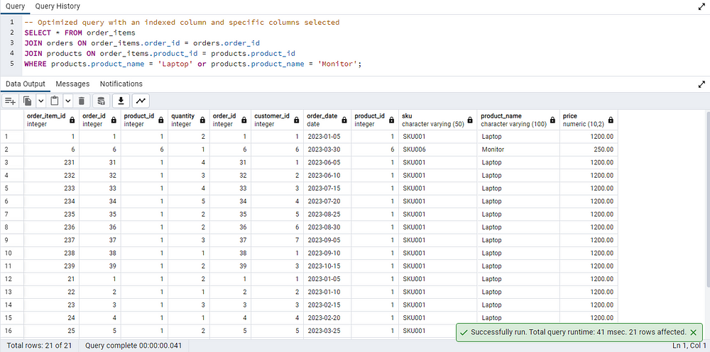
The total query runtime is 41 msec. This can be optimized by using a specific number of columns that are needed and by using Indexing in the query.

Solution 1: Use SELECT with Specific columns instead of SELECT *

It’s crucial to consider whether this extensive data retrieval is necessary. Opting for specific column names in the SELECT statement, as demonstrated in the example, reduces the amount of data fetched.

-- Optimized query with specific columns selected 
SELECT 
order_items.order_item_id, orders.order_id 
FROM order_items

This approach accelerates query execution because the database only needs to retrieve and deliver the requested columns, not the entire set of table columns.

Solution 2: Indexing

An index serves as a data structure designed to enhance the efficiency of data retrieval operations within a database table. When implementing a unique index, distinct data columns are established without any overlap.

In addition to facilitating quicker data retrieval, indexes also contribute to optimizing query performance by serving as a roadmap for the database engine.

Use the following flow chart as a guide to query indexing.

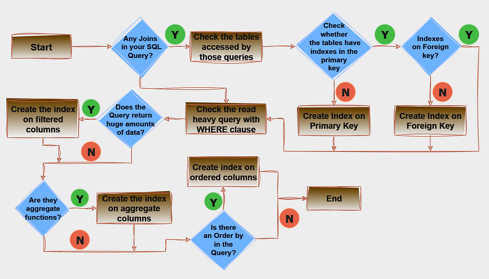
However, it’s essential to strike a balance, as excessive indexing can lead to increased storage requirements and maintenance overhead. Regular monitoring and strategic indexing are key aspects of maintaining a well-performing database.

-- Adding an index on the 'product_name' column of the 'products' table 
CREATE INDEX idx_products_name ON products(product_name); 

-- Optimized query with an indexed column and specific columns selected 
SELECT 
order_items.order_item_id, orders.order_id, orders.order_date, products.product_name, order_items.quantity 
FROM order_items 
JOIN orders ON order_items.order_id = orders.order_id 
JOIN products ON order_items.product_id = products.product_id 
WHERE products.product_name = 'Laptop';

A new index, labeled, is created on the product_name column within the products table. This index is beneficial for optimizing query performance, particularly when filtering based on the product name.

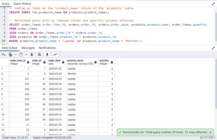
The total query runtime was reduced to 25msec which is almost half of the previous query runtime.

2. Caching Mechanisms

By implementing a caching strategy for your database, you can enhance database performance, availability, and scalability at a minimal cost, depending on your approach.

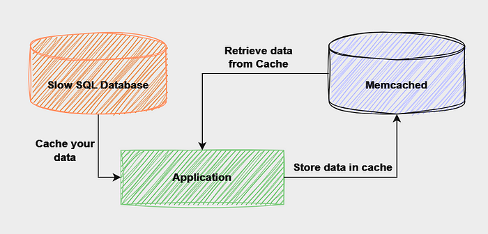
We can use a caching strategy that stores frequently accessed data in memory to improve response time in read-heavy operations. I have used Memcached with Python which is a caching solution to implement a caching mechanism on our database.

from pymemcache.client.base import Client 
import psycopg2 
import json 

# Connect to Memcached 
memcached_client = Client(('localhost', 11211)) 

def fetch_data_from_database(query): 
  # Implement your database connection logic (e.g., using psycopg2)
  # Execute the query and fetch data from the database
  # ... 

# Convert the result to a JSON string 
  result_json = json.dumps(result) 

# Store the result in Memcached with a key 
  memcached_client.set('cache_key', result_json, expire=3600) # Cache for 1 hour

return result 

def get_data_from_cache_or_database(): 
  # Attempt to retrieve data from the cache 
  cached_data = memcached_client.get('cache_key') 

if cached_data: 
    # If data is found in the cache, return it
    return json.loads(cached_data.decode('utf-8')) 
  else: 
    # If data is not in the cache, fetch it from the database 
    data_from_db = fetch_data_from_database('SELECT * FROM order_items;') 
    return data_from_db 

# Example usage 
result_data = get_data_from_cache_or_database()

The pymemcachelibrary is used to interact with the Memcached server.

The fetch_data_from_database() function fetches data from the database, converts it to JSON, and stores it in Memcached with a key ('cache_key').

The get_data_from_cache_or_database() function attempts to retrieve data from the cache. If data is found, it's returns; otherwise, it's fetched from the database.

Keep in mind that caching is particularly beneficial for data that remains relatively static and can be securely held in memory for a defined duration. It is crucial to implement cache invalidation strategies to prevent outdated information from introducing inconsistencies in your application.

3. Denormalization

Denormalization serves as a database optimization strategy where redundant data is introduced into one or more tables, aiming to eliminate the need for expensive joins in a relational database.

Consider a scenario where you often need to retrieve information about products along with their order details, customer information, and order item quantities. In a normalized form, you might have to perform multiple joins to get this information.

In a denormalized schema, you might create a new table that combines information from the products, orders, customers, and order_itemstables.

CREATE TABLE denormalized_inventory (
    order_item_id serial PRIMARY KEY,
    order_id INT,
    order_date DATE,
    customer_id INT,
    customer_first_name VARCHAR(50),
    customer_last_name VARCHAR(50),
    customer_email VARCHAR(100),
    product_id INT,
    product_sku VARCHAR(50),
    product_name VARCHAR(100),
    product_price DECIMAL(10, 2),
    quantity INT
);

With this denormalized table, you can perform reads that involve product details, order details, and customer information without the need for multiple joins.

Optimized Read Scenario

-- Retrieve information about products, orders, and customers without multiple joins
SELECT * FROM denormalized_inventory WHERE product_name = 'Laptop';

It’s crucial to evaluate the specific requirements and usage patterns of your application to determine whether denormalization is the right approach and how much to denormalize. Regular monitoring and testing are essential to ensure that the chosen denormalization strategy continues to meet the performance and consistency needs of your application.

4. Partitioning Tables

Table partitioning is a database design method that entails breaking down a sizable table into smaller segments, known as partitions, each storing a distinct subset of the initial data. These partitions can be established using specific columns, like dates or value ranges.

Employing partitioning allows database systems to efficiently exclude irrelevant partitions during queries.

Partitioning in PostgreSQL provides different methods like:

• Range Partitioning
• List Partitioning
• Hash Partitioning

I will provide an example of List partitioning for our warehouse_inventorydatabase.

We will generate separate tables to depict each partition, and each partition will encompass a distinct product category. To illustrate, we will establish three partitions: “Computer Accessories,” “Camera Accessories,” and “Wearables.

-- Assuming there is a 'category' column in the 'products' table
CREATE TABLE products (
    product_id serial PRIMARY KEY,
    sku VARCHAR(50) UNIQUE,
    product_name VARCHAR(100),
    price DECIMAL(10, 2),
    category VARCHAR(50) -- Assuming a 'category' column
);

-- Create partitions for different product categories
CREATE TABLE electronics PARTITION OF products
    FOR VALUES IN ('Computer_Accessories');

CREATE TABLE clothing PARTITION OF products
    FOR VALUES IN ('Camera_Accessories');

CREATE TABLE furniture PARTITION OF products
    FOR VALUES IN ('Wearables');

List partitioning enables the explicit definition of distinct values for individual partitions. This approach proves beneficial when data can be classified into separate and non-overlapping sets.

Insert the data into their respective partitions as given below.

INSERT INTO products (sku, product_name, price, category)
VALUES ('ELEC001', 'Gaming Mouse', 800.00, 'Computer_Accessories');

INSERT INTO products (sku, product_name, price, category)
VALUES ('CLOTH001', 'Camera Lens', 20.00, 'Camera_Accessories');

INSERT INTO products (sku, product_name, price, category)
VALUES ('FURN001', 'Fitness Tracker', 500.00, 'Wearables');

During read operations, SQL will automatically retrieve information from the respective partition as specified by the WHERE clause.

-- Retrieve Computer_Accessories products
SELECT * FROM products WHERE category = 'Computer_Accessories';

5. Materialized Views

A materialized view in a database stores the actual results of a saved query as a physical table. This storage enables faster access compared to recomputing the view each time it is queried. Essentially, a materialized view acts as a cache, providing quick access to precomputed data. If a regular view is a saved query, a materialized view goes further by storing both the query and its results.

Key points about materialized views:

• Efficiency in Querying: Materialized views eliminate the need for recomputation when referenced in a query, resulting in faster access to the stored results.
• Indexing Capabilities: Because materialized views are stored like tables, indexes can be built on their columns, further improving query performance.

Now, let’s create a materialized view to show the total quantity of each product sold:

CREATE MATERIALIZED VIEW product_sales_summary AS
SELECT
    p.product_id,
    p.product_name,
    SUM(oi.quantity) AS total_quantity_sold
FROM
    products p
JOIN
    order_items oi ON p.product_id = oi.product_id
GROUP BY
    p.product_id, p.product_name;

REFRESH MATERIALIZED VIEW product_sales_summary;

In this example:

• The materialized view named product_sales_summaryaggregates the total quantity of each product sold by joining the products and order_items tables.
• The REFRESH MATERIALIZED VIEW statement is used to refresh the materialized view with the latest data. You can run this statement periodically or as needed to update the materialized view.

Now, you can query the materialized view to get the total quantity of each product sold:

-- Query the materialized view
SELECT * FROM product_sales_summary;

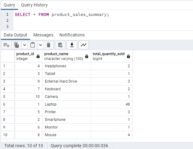
Materialized views offer the capability to define complex data transformations using SQL and delegate the maintenance of results to the database, essentially creating a “virtual” table.

6. Read Replicas

Read replicas are exact copies of the primary (master) database that are used to distribute read queries and reduce the load on the primary database. These replicas are synchronized with the primary database but are dedicated to handling read operations.

• Load Balancing: Read replicas help distribute read queries across multiple database instances, balancing the load and preventing the primary database from being overwhelmed by read-heavy queries.
• Improved Read Performance: The primary database can focus on handling write queries by offloading read queries to replicas.
• High Concurrency: Read replicas allow high concurrency as multiple queries can be executed concurrently across different replica instances, providing better scalability.

• Replication Lag: There may be a slight replication lag between the primary database and read replicas. This lag needs to be considered when ensuring data consistency.
• Configuration and Monitoring: setting up replication, monitoring replication lag, and adjusting the number of replicas based on workload changes are crucial to ensuring the effectiveness of read replicas.
• Applicability to Query Patterns: If the workload is primarily write-heavy, the benefits of read replicas may be limited.

7. Hardware Optimization

Consider upgrading the system’s hardware components, such as increasing CPU, RAM, storage, or other relevant resources.

Since we are using PostgreSQL, we can boost its performance by adjusting the shared memory buffer size, specifically the shared_buffers parameter. Shared buffers in PostgreSQL serve as a cache for frequently accessed data, reducing the necessity to read data from the disk.

-- Upgrading the database server's RAM for PostgreSQL
ALTER SYSTEM SET shared_buffers = '16GB';

This determines the amount of memory allocated to the shared memory buffer pool. While the shared_buffersparameter is typically specified in the postgresql.conf configuration file, using the **ALTER SYSTEM SET** command allows for dynamic configuration changes without requiring a full restart of the database server.

8. Connection Pooling

Instead of opening and closing connections for each user or request, a pool of connections is maintained. This reduces connection overhead, improves response times, and optimizes resource utilization.

Using a connection pooling library, such as HikariCP in Java, allows for easy configuration and integration into applications. Proper monitoring, tuning, and closing connections after use are essential considerations for effective connection pooling.

9. Monitoring and Tuning

Step 1: Monitoring

• Use tools like pg_stat_statements to analyze query performance.
• Utilize monitoring solutions like pgAdmin or Datadog to track metrics such as CPU usage, memory consumption, and I/O operations.

Example Query:

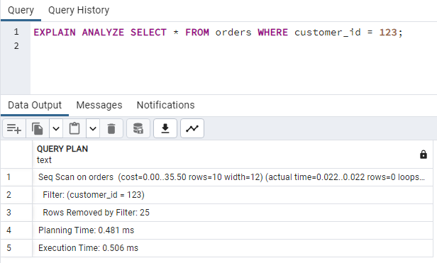
Let’s say you have a query that retrieves data from a table named orders:

SELECT * FROM orders WHERE customer_id = 123;

Use EXPLAIN ANALYZE to get insights into the query execution plan and identify potential bottlenecks.

Step 2: Tuning

After monitoring, you identify that the query performance is affected by the lack of an index on the customer_id column.

• Create an index on the customer_idcolumn to speed up the retrieval of relevant rows as we discussed at the beginning of this article
• Adjust PostgreSQL configuration parameters, such as shared_buffersor work_mem, based on observed metrics.

Create an index on the customer_idcolumn:

CREATE INDEX idx_customer_id ON orders(customer_id);

Ensure that statistics are up to date:

ANALYZE orders;

Configuration Adjustment:

Modify the shared_buffersparameter in postgresql.conf:

# shared_buffers = 128MB
shared_buffers = 256MB

Step 3: Continuous Monitoring and Iterative Tuning

After applying tuning measures, monitor the system to ensure that the changes have the desired impact. You must regularly check performance metrics and logs.

Wrapping Up

In conclusion, optimizing SQL databases for large datasets is vital to sustaining efficient application performance. These strategies empower systems to handle increased workloads, minimize downtime, and ensure scalability, addressing the challenges posed by expanding datasets and enhancing the overall sustainability of the database infrastructure.