Cookpad Kitchen

The job of a search relevance engineer frequently involves (as you probably already know if you’re reading this!) tuning different relevance signals for different search queries, to optimise both the returned search results as well as the result order.

These relevance signals could for example be different matching strategies against different document fields, or they could be other arbitrarily complex ones.

A concrete basic example would be to consider documents consisting of just a few fields, say “Title” and “Ingredients”

The job of the relevance engineer using Elasticsearch would then be to construct basic text queries against both the two text fields, the “Title” and the “Ingredients” field, along with perhaps phrase queries against both of those fields. Each of those 4 sub-queries would be scored under BM25.

This would in turn give the engineer 4 signals to assign weights to.

The relevance engineer would then have to, taking also into account the magnitude of the scores of these different sub-queries, assign different weights to all these scores so that when summed up together, the resulting ordering has more relevant documents further up the top.

For example, they could determine that while the sub-query that matched the “Title” field on average has double the score value of the sub-query that matched the “Ingredient”, a match on the title is much more important for searchers, so they would assign a weight that ends up boosting the score coming in from matching the title.

In a simple example like this, it’s quite easy to reason about the importance of different fields to search for users. But even in this toy example, it’s not immediately easy to reason about how important different matching strategies are.

Would matching your query as a phrase in the recipe’s ingredients be less or more important than matching the query against the title as separate terms?

Then simply imagine adding more fields, such as a “Hashtag” field, how important is matching that versus matching the title? What about another 10 text fields?

Oh, and we also think that recent documents are probably more relevant to searchers, we should definitely boost newer documents! But by how much?

How do we solve this mess? Let’s try to learn these values instead of hand-tuning them!

What does “learning to boost” mean?

“Learning to Boost” is a name that has been used to refer to techniques that leverage data to optimise scoring, under Elasticsearch or other Lucene-based systems, by adjusting how different signals contribute to the final score of a retrieved document.

When referring to signals, in this case, we’re referring to things that we express as sub-queries that contribute to the individual final document score for a given query. And as mentioned these could be text queries or, they could be any other arbitrary Elasticsearch/Lucene query that we can express (such as, for example, a function query that assigns a score value according to a date value present on the document).

What data can you use to do this? You might already have access to judgement lists produced by domain experts about some of your queries. Or you are building them by either implicit or explicit feedback (some information on judgement lists).

But even if you’re not already doing that, in most situations you’re already keeping track of what your searchers are clicking on out of the results that they’re being shown, and as mentioned that can serve as implicit feedback about which results are the most relevant.

Using that data, you learn values that balance these different signals better than you would as a human trying to balance potentially hundreds of different scores for thousands of different queries.

And it might not even be the end of your journey. You could be already utilising a two-stage approach to re-rank your top results according to more complex logic (eg. with an ML-based re-ranker).

But if your initial result lists are several thousands of documents long, then even re-ranking on the top few hundred results could be missing important results, simply because your manual tuning didn’t bring them far enough up in the initial retrieval (by, for example, giving too much importance to a field that’s not actually the only one that matters).

Optimising the initial retrieval step then isn’t superfluous but highly complementary to your re-ranking.

Why did we believe we needed this at Cookpad?

Cookpad is trying to help cooks find the best recipe to cook today, out of millions of recipes constantly coming in from our huge community.

Our recipe documents hold a lot of information that searchers might want to match against. They could be looking for a dish name in the title of a recipe, or for an ingredient in the ingredient list. Or they could be looking for a special treat for a specific holiday, which they would be able to find in the description associated with a recipe.

We also directly or indirectly know a lot about the quality of a recipe submitted to our platform. We can have heuristics about how well it’s been composed, how nice the associated image looks, and how popular each recipe is with other users, in what ways they’re interacting with it.

At the same time, we believe that for our user’s freshness is important as it, well, keeps things fresh! Seeing new things is always inspiring in itself, but it also allows you to see how the community around you is adjusting to current food trends, the upcoming holidays, or the items of the season.

This means we have a lot of different things to balance, and for some of these signals, we’re not even certain of how much our searchers value them!

To make matters even worse, we operate in tens of different countries. Each with its own specific user behaviour and preferences, to the point where treating them uniformly, would mean that search performance would suffer.

Learning to boost could be our solution to the manual tuning we have been doing.

Learning to Boost at work — detailed example

If you’ve done relevance tuning in the past, you’ll be familiar with the goal of this process. However, if you’re new to this domain, an illustrated example could help.

So we’ll do just that, using just a couple of subqueries/fields although in practice you’ll likely have tens if not hundreds.

The way Elasticsearch scoring works is that each individual subquery’s score is multiplied by a boost/weight value. These scores are added together to compute a final document score for a given query. The documents are then ranked in descending order of the total score.

Here’s the result list for a hypothetical recipe search. This is a simplified search example, for sake of demonstration. You can see that each recipe document’s score is determined by multiplying the BM25 text query score for subqueries targeting each of the two text fields with a boost value and summing these together.

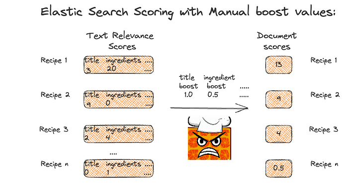
Figure 1: Example using Manual boost values.

As seen above, recipe 2 is ranked second. However, from inspecting the results for this search query, we might believe Recipe 2 is the most relevant result. This means that ordering isn’t ideal, and we can try to tweak it to improve things.

We might have the intuition that the title conveys a lot of relevance information, and we should decrease the amount that the ingredients contribute.

And indeed if we adjust our boost values and do the subsequent math, we can achieve the ideal ordering we were after.

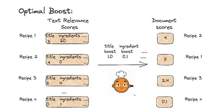
Figure 2: Example using Optimal boost values.

A “learning to boost” process aims to do the above across more than just one example query. It tries to optimise these values so that the amount of queries and documents in the right order are maximised.

It does so in a more automated fashion. And removes some of the subjectivity in the previous process — remember that in the previous example we inspected the results by hand to come to our own assessment of how to adjust the boost. That’s an approach that’s hard to scale to many queries!

Breaking it all down:

So let’s follow the whole process we followed at Cookpad for doing this sort of tuning. Roughly, we have the following steps:

Figure 3: Learning to Boost Architecture

Here, data collection refers to collecting interaction data that will drive our optimization process, while feature parsing refers to collecting all the different scores for all the query/document pairs that will participate in our tuning process. Model training and evaluation are about performing the actual optimization process and evaluating the outcome.

Data Collection:

Figure 4: Data Requirements

The first step is collecting data to optimise on. The data required for this process is essentially the same data that can be used for Learning To Rank approaches.

In our case we used interaction data to build judgement lists; i.e., searchers in the app interacting with recipes through search results. To do this we took a very basic approach.

We first picked a list of popular or important queries. Specifically, we chose to focus on our top 100 queries, which for us represent a significant percentage of our overall search volume.

Then, for each of these queries, we constructed a list of the most common recipe results.

For each of those recipe documents, we calculated a success rate. There are many ways you can define a success rate, and the choice depends on your domain and what you want to optimise for. This could be, for example, clicking through to the page, dwelling on the page for a minimum duration, or deep scrolling (reaching some point on the page), or taking a positive action on the page (bookmarking, liking, etc.), and so on.

This simple scheme allowed us to get, for each of our queries, a list of recipe documents ordered by user preference (most preferred to least preferred) by considering more successful documents as more preferred for this query.

We also probably want to define some sort of heuristic or threshold of how many times a document has been shown to users, or how many times the document has actually been examined and visited for this query, and not including documents that fall under this threshold in your lists.

We went with a simple threshold ourselves.

Implicit vs Explicit Judgments:

To create the relevance labels for training data we could use either implicit or explicit judgments.

To get explicit judgments, we would ask domain experts to label the data manually which increases effort, coordination overhead and probably costs, but these judgments are less prone to position bias.

When leveraging implicit feedback, as we did here, user interactions with search results are used to generate relevance labels. In our case, These kinds of labels are quite easy to get after you determine a certain scheme and provide a bigger set of data (covering more documents and more queries than you could otherwise afford to). However, because they are dependent on your displayed result sets, they come with the inherent position and presentation biases.

Using our lists to tune by transforming into pairs:

We decided to go with a pairwise approach to tune on. A pairwise approach in learning to rank refers to tuning based on a pair of documents at a time, where one item out of the pair is preferred over the other for a given query.

In order to construct these pairs, we very simply sampled documents from our ordered lists. We can just pick two items in a list, and consider the one that’s placed higher up as the preferred item in the pair.

This should serve as a good baseline to get started, but there are a lot of shortcomings with such a simple approach that you will probably want to consider adjusting for.

You can for example easily notice that what we outlined pays the same amount of attention to a pair where the documents are close in terms of success, and a pair where one document is almost always preferred to the other.

It also pays the same amount of attention to any document in a list that happened to be displayed and interacted with enough to be above the threshold (i.e., any document that made the list).

Finally, it pays the same attention to frequent vs rare queries, because the data set you’re generating isn’t biased in any way towards the more frequent ones.

So if you invest heavily in this process, you’ll probably want to account for these problems by adjusting how you pick which pairs to include in your dataset / how much attention you pay to them during subsequent steps.

Pointwise vs Pairwise:

Figure 5: Pointwise vs Pairwise LTR

The pointwise LTR method is the simplest form of a ranking model, considering each document independently of the other in the loss function. This model takes a single document and query as input at a time and tries to predict how relevant the document is to the query. As such, there’s nothing that explicitly concerns ranking here, only a relevance score being predicted.

In the pairwise approach, a pair of documents is examined at a time, and training aims to minimise the observed inversions from the ideal ordering (i.e., when a document that should be less preferred has a higher score than another one).

Pairwise approaches generally work better in practice than pointwise approaches because predicting relative order is closer to the nature of ranking than predicting class labels or relevance scores. And as a method, it doesn’t impose on you the requirement of having very accurate relevance judgements/scores for a lot of your documents and queries.

Feature parsing:

After building up the preference pairs part of our dataset, the next step is to retrieve the “feature” values for the documents to complete the training dataset. These would be the different score values for a given document for each of our queries.

To do this, you could opt for various different approaches. If you’re using ES as we are, you could opt to use the LTR plugin which would make retrieving these values easier by structuring all this information and returning it along with your documents when you’re going back and re-running your queries to get these values.

You could also forgo any external dependencies — as we did — and for example, parse the Elasticsearch explain output of your query responses.

An important consideration is whether you can effectively retrieve all these during this optimization process, or if you should be proactively logging all this information when your queries are being run in your production setting. Being proactive could look like extra work, but having these already stored (after all, they were likely being calculated during retrieval) could lessen the required load during this training. It could also save you the headache of capturing the at-the-time state of your document in case you are dealing with documents with changing values!

But keep in mind that having detailed logging of previous searches might not be enough if you’re also introducing new score components/features along with this tuning.

Caveat — what can you actually tune?

Before embarking on tuning all the weights on your various sub-queries, you have to consider whether the ratios and magnitudes of their individual scores are all in line with each other.

Take our example — we are going to tune the weights of sub-queries that target 2 of our fields, “Title” and “Ingredients”. These fields will have similar lengths and similar term distributions. Therefore if we have 2 of those queries, the resulting score for a match will be fairly similar. It might range in magnitude between short and long queries, but it’s still going to be within the same range for a given query.

Or the nature of your constructed queries and fields could dictate that for a given query, a great score for a query targeting one field is statically proportional to a great score for another query targeting another field (perhaps because the lengths of the fields are vastly different and you’re not any field length normalisation).

Or, even, the nature of your dictates that the range of scores is within a standard range regardless of the search query at hand, as could be the case if you’re doing mostly filter queries and ranking by a PageRank score and a component based on document recency.

These examples would work out fine.

The trouble would start when you’re trying to combine some of these together. Text relevance scores are generally unbounded and wildly different between different query lengths and fields.
Trying to decide how much a score like that should contribute for all queries, versus another score that always ranges between 0 and 1, is not going to work out!

Even worse, if you pick a small query sample to tune on you might not even realise the damage you’re doing to your ranking algorithm.

So be careful!

The obvious solution to any such problems would be to normalise all your sub-scores in a certain range. Unfortunately, it’s not something that you can easily do if you’re using ES like we are (you can follow the discussion on this subject here).

Data-driven optimization:

Now comes the part where we try to learn the optimal weights for all the things that contribute to scoring.

Remember, all these scores are multiplied by the corresponding weights and added together to produce a final score for a given document. So the final score is a linear combination of all the individual subquery scores. So our process needs to somehow optimise for this linear combination. Specifically, it needs to determine weights so that given a set of preferences (which express that “document A is preferred to document B for query Q”) it maximises the number of preferences that it ends up satisfying after the weights are adjusted.

Treating this problem as a sort of regression that yields a linear model gives us the framework on how to tackle this problem.

Specifically, we can transform our preference pairs in a way that allows us to treat this as a logistic regression problem.

Pairwise Transform Trick:

For the transformation, we do the following for each pair of preferences [q, (docA > docB)] (where q is the query at hand, and docA and docB are documents where one is preferred over the other as a result for this query):

• Randomly decide if you should flip the pair so that the preferred document comes second (it will help in a subsequent step)
• Subtract the “feature” values for the pair.
• If the first document was preferred, assign the label 1 otherwise assign the label 0.

Figure 6: Pairwise Transformation

So now you have a single linear combination of “feature” values, and a single label to predict per pair.

By running a linear regression optimization on this and getting the subsequent model, we’re going to be optimising for these coefficients, in a way that aims to satisfy our ideal ordering, and then we can map these back to our different query weights.

To give a little theoretical justification for using the logistic regression model on pairwise data, let us look at an example below.

Figure 7: If L_a > L_b, recipe a is more relevant than recipe b.

Supposing we have two recipes a, b from the search result list, in the first two equations we can see how the scores are calculated for these recipes in a pointwise fashion. After taking the difference of the feature values in the last equation we can get the pairwise values. In both of these arrangements, the coefficient values remain the same, which means we can use these coefficient values from the pairwise approach the same way as in the pointwise approach and plug these values in elasticsearch as boost values.

Linearity constraint:

As it should be obvious, by modelling our problem this way we’re introducing a constraint to the queries that we can tune the weight for. Namely, we can tune only the weight that is multiplied by the score of sub-queries and added to the total score of the document. This means that if you combine your queries using more complex query structures (an ES example would be using multi-match queries with best_fields) then you won’t be able to tune the inner weights/boosts, but only the top level one that is applied to this nonlinear combination of scores.

Model Training:

After applying the pairwise transformation to the dataset, solving the optimization problem by training the logistic regression model is straightforward and a lot of off-the-shelf libraries can be used for that.

We specifically used scikit-learn.

Another thing to remember while training the model is to restrict the values of the coefficients to non-negative as in Elasticsearch boosts values cannot be negative.

Evaluation:

Post-training, you’ll want to evaluate the generated model in terms of how closely it fits the data you fed into it, and also how well the generated values work for your search when transferred over to your ranking algorithm.

For offline evaluation, we checked on the typically used metrics of Area Under Curve (AUC), precision, and recall scores.

As mentioned earlier, our dataset was built from our top 100 queries in recent months.

We used 80 of those for our training (representing millions of searches), and we used the other 20 to evaluate our model.

Since the loss function of the logistic regression model is cross-entropy loss, which is not directly optimising the search metrics that take into account the position of the documents the question that arises here is how can AUC help us in evaluating the ranking model.

In practice, we have seen the logistic regression metrics (precision, recall, AUC, etc) and ranking metrics (nDCG, MRR) generally agree until the AUC score is very close to 1.

For our online evaluation, we generally focus on Click Through (CTR) and session success rates, and for any changes coming in from this process we would set up an A/B experiment to make sure that these adjustments transfer to the main task at hand.

Deployment:

Deploying the outcome of the optimization problem should be rather easy, as there’s no complex process taking place on query time. We just have to go and update the different values used as boosts. Since we’re using ES ourselves, we just had to update the values in the ES DSL queries we’re running when they’re being generated. If you are using search templates, you should update those instead.

After deploying the model we can easily repeat this process when we have more data coming in from searches (allowing us to adjust our weights to serve more diverse or more current queries), or when we add new things that can contribute to scoring to our queries (and avoid the headache of balancing the contribution of anything new with what’s already there).

Takeaways:

The outlined learning-to-boost approach is an easy way to get started with tuning weights in a data-driven way and moving away from doing all your tuning manually.

And thus, it can be a way to improve how your search performs in terms of metrics in itself.

It can also serve as a powerful baseline for more complex re-ranking schemes like Learning to Rank.

Particularly for Learning to Rank, it can be a great stepping stone to that, as it can inform engineers of related techniques and the value that it could bring, while not requiring any new external systems or even any technology to be adopted besides what should already be in use in your search system.

Additionally, apart from any immediate impact on your search performance, the weights you get out of an automated process like this can be a source of valuable information about the preferences and biases that searchers have, driving you to design not just your search experience but also your product to either serve these preferences better or correct for these biases!

At the same time and directly related to that point, you need to be aware that if you optimise for search preferences you could be actually going against your stated product or business goals.

In this case, while you can’t blindly bring your automatically tuning weights to your search, the revealed biases can again drive how you design your product and also can help you discover useful “guardrails” for your search.

As an example, imagine if searchers always prefer cheaper products, which for the business have a lower profit margin. If you notice that your automated tuning ends up placing big importance on products having the lowest price, you might not want to blindly bring this to your search, despite this improving your typical search metrics! Instead, if you haven’t implemented this already, it might immediately highlight that you would be greatly served by tracking other metrics relating search to revenue and thus keep you from making search changes in the wrong direction.

I would like to acknowledge the members of the Search Science team at Cookpad who all contributed to this work: Apostolos Matsagkas, Orgil Davaa, Akbar Gumbira and Matthew J Williams. I would also like to acknowledge Nina Xu for answering my queries regarding the LTB approach.

Resources: