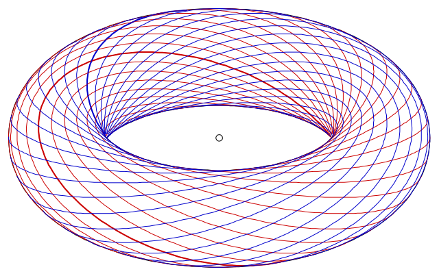
Image from Wikimedia Commons

These curves defined by very simple equations are shrouded in mystery and elegance. In fact, the equations describing them are so simple that even high-school students would be able to understand them.

However, a ton of simple questions about them remain unsolved despite tenacious efforts by some of the greatest mathematicians in the world. But that’s not all. As you will soon see, this theory connects various important fields of mathematics because it turns out that elliptic curves are more than just plane curves!

Let’s grab a cup of coffee and start from the beginning.

Introduction and Motivation

In mathematics, we often solve problems by stating them in a different setting than they originally occurred in. An example of this is that some geometric problems can be turned into algebraic problems and vice versa.

A classical problem going back thousands of years is whether a positive integer n is the area of some right triangle with rational side lengths, that is such that the lengths of all three sides are expressible as fractions of whole numbers. In this case, n is called a congruent number). For instance, 6 is a congruent number because it is the area of the right triangle with side lengths 3, 4 and 5.

In 1640, Fermat famously proved that 1 is not a congruent number. He did so using his famous method of proof by infinite descent.

As the amazing mathematician, Keith Conrad notes about the result:

This leads to a weird proof that √2 is irrational. If √2 were rational then √2, √2 and 2 would be the sides of a rational right triangle with area 1. This is a contradiction of 1 not being a congruent number!

Since Fermat’s proof, the hunt for proving or disproving that numbers are congruent has been ongoing.

Amazingly, one can show by elementary methods that for each triple of rational numbers (a, b, c) such that a² + b² = c² and 1/2 ab = n, we can find two rational numbers x and y such that y² = x³ - n²x and y ≠ 0 and conversely for each rational pair (x, y) such that y² = x³ - n²x and y ≠ 0, we can find three rational numbers a, b, c such that a² + b² = c² and 1/2 ab = n.

That is, right triangles with area n correspond exactly to rational solutions to the equation y² = x³ - n²x with y ≠ 0 and vice versa. A mathematician would say that there is a bijection between the two sets.

Therefore, a rational number n > 0 is congruent if and only if the equation y² = x³ - n²x has a rational solution (x, y) with y ≠ 0. For example, since 1 is not congruent, the only rational solutions to y² = x² - x have y = 0.

For the interested reader, the exact correspondence is the following.

If we try this correspondence on the triangle with side lengths 3, 4, and 5, and with area 6, then the corresponding solution is (x, y) = (12, 36).

To me, this is absolutely amazing. One starts with a problem in number theory and geometry and through algebra, transforms it into a problem about rational points on plane curves!

The equation y² = x³ - n²x is an example of an elliptic curve.

Elliptic Curves

In general, if f(x) denotes a third-degree polynomial with a non-zero discriminant (i.e. all the roots are distinct), then y² = f(x) describes an elliptic curve except for one important addition to this object, namely what is called a “point at infinity”.

Basically, a point at infinity is a point where parallel lines can meet. It is out of the scope of this article to go into projective geometry to proper define it but this is a wonderful and exciting subject that I strongly encourage you to look up.

Now, by a minor algebraic miracle, it turns out that we can make a suitable (rational) change of coordinates, and get a new curve on the form y² = x³ + ax + b such that rational points on the two curves are in one-to-one correspondence. The second transformed curve however is typically easier to work with.

Because of this, we sometimes assume that an elliptic curve is on this form and so from now on we will assume that too, that is, when we say “elliptic curve”, we mean a curve on the form y² = x³ + ax + b together with a point 𝒪 at infinity.

Throughout this article, unless otherwise stated, we’ll assume that the coefficients a and b are rational numbers.

Elliptic curves take on two typical shapes which are graphed below.

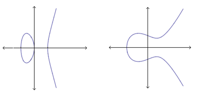
Image from Wikimedia Commons

However, if we consider x and y as complex variables, the curves will look entirely different. In fact, they will then take the form of a complex torus or doughnut!

So why do we study elliptic curves and what can we do with them?

First of all, many number theoretic problems can be translated into problems about Diophantine equations, secondly, it turns out that elliptic curves are related to discrete geometric objects called lattices and deeply connected to some very important objects called modular forms which are certain extremely symmetric complex functions with a lot of number theoretic information in them.

Actually, the connection between elliptic curves and modular forms turned out to be the key to proving Fermat’s Last Theorem which Andrew Wiles achieved in the 90s through several years of intensive work on this connection.

The story about this quest and the proof of the Theorem is in my opinion one of the most beautiful pursuits in all of science - unfortunately, as pointed out by my friend

, the margin in this Medium post is too narrow to contain it!

So I guess I’ll have to write another article.

Elliptic curves are also used in cryptography to encrypt messages and online transactions.

The most important feature of them, however, is the mind-blowing fact that they are more than just curves and more than just geometry. In fact, they have an algebraic structure on them called an Abelian group structure with respect to a cool geometric operation - a kind of geometric addition rule for how to add points on the curve together.

If you don’t know what an Abelian group is, you can think about it as a set of objects with an operation defined on them such that they have the same kind of structure as the integers with respect to addition (except they can be finite).

More specifically, for a group with the operation *, it needs to be stable with respect to the operation (i.e. if a is in the group and b is in the group, then a * b is in the group), there is an identity element e (0 for the integers) such that a * e = a for all elements a in the group, and for each element a, there is an inverse element c, such that when you operate them together you get back the identity element (a * c = e). Furthermore, the group operation has to be associative i.e. a * (b * c) = (a * b) * c. That is, it doesn’t matter which elements you add together first. If the commutative law holds ( i.e. a * b = b * a) then the group is called an Abelian group.

Examples of Abelian groups are:

1. The integers ℤ with respect to the operation +.
2. The action of rotating a square clockwise by 90 degrees
3. Vector spaces with vectors as elements and vector addition as the operation

The fancy terminology for a curve with an Abelian group structure is Abelian variety.

What is so amazing about elliptic curves is that we can define an operation (let’s denote it ⊕) between rational points on them (that is, both the x and y coordinates are rational numbers) such that the set of those points on the curve becomes an Abelian group with respect to the operation ⊕ and with identity element 𝒪 (the point at infinity).

Let’s define the operation.

If you take two rational points on the curve (for example P and Q) and consider a line through them, then the line intersects the curve at another rational point (possibly the point at infinity). Let’s call this point -R.

Now, because the curve is symmetric about the x-axis, we get another rational point R when we reflect -R about it. There is a drawing of this below.

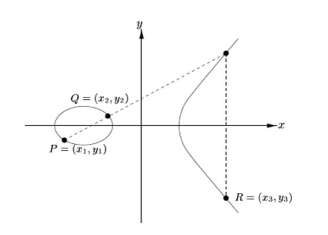
Addition rule for elliptic curves - image from Wikimedia Commons

This reflected point (R in the above image) is the addition of the two aforementioned points (P and Q above). We can write P ⊕ Q = R.

One can prove (and this is actually not easy) that this operation is associative, which is really surprising, at least to me. Also, the point at infinity acts as a (unique) identity for this operation and each point has an inverse point (which is just the point you get by reflecting about the x-axis). It is also Abelian (i.e. P ⊕ Q = Q ⊕ P).

The Mystery

It turns out that two different elliptic curves can have vastly different groups associated with them. An important invariant that in some sense is the most defining feature is what is known as the rank of the curve (or group).

A curve can have a finite or an infinite number of rational points on them. This can be hard to handle, so what we are interested in, is how many points we need in order to generate all the others by the aforementioned addition rule. These generators are called basis points.

The rank is a dimensionality measure like the dimension of a vector space and indicates how many independent basis points (on the curve) have infinite order (i.e. we can keep adding it without getting our starting point back). If the curve only contains a finite amount of rational points on it, then the rank is zero. There is still a group but it is finite.

Calculating the rank of an elliptic curve is notoriously difficult but we have a nice result due to Mordell which tells us that the rank is always finite. That is, we only need a finite amount of basis points in order to generate all the rational points on the curve.

One of the most important and interesting problems in number theory is called the Birch and Swinnerton-Dyer Conjecture and it is all about the rank of elliptic curves. In fact, it is so difficult and important that it is one of the Millenium Problems.

You actually get a million dollars if you solve it!

Finding rational points on elliptic curves with rational coefficients is hard. One way to approach this is by reducing the curve modulo p where p is a prime number. This means that instead of considering the rational solution set of the equation y² = x³ + ax + b, we consider the rational solution set of the congruence y² ≡ x³ + ax + b (mod p) where for this to make sense we might have to clear denominators by multiplying by an integer on both sides.

So we are considering two numbers with the same remainder when divided by p to be equal in this new space. The great thing about this is that now there are only a finite number of things to check. Let’s denote the number of rational solutions to such a reduced curve modulo p, by Np.

In the early 1960s, Peter Swinnerton-Dyer used the EDSAC-2 computer (not exactly a Macbook!) at the University of Cambridge Computer Laboratory to calculate the number of points modulo p on elliptic curves with known rank. He worked together with the mathematician Bryan John Birch in understanding elliptic curves and after the computer had crunched a bunch of products of the form

for growing x, they got the following output taken from data associated with the curve E: y² = x³ − 5x (as an example). I should note that the x-axis is really log log x and the y-axis is log y.

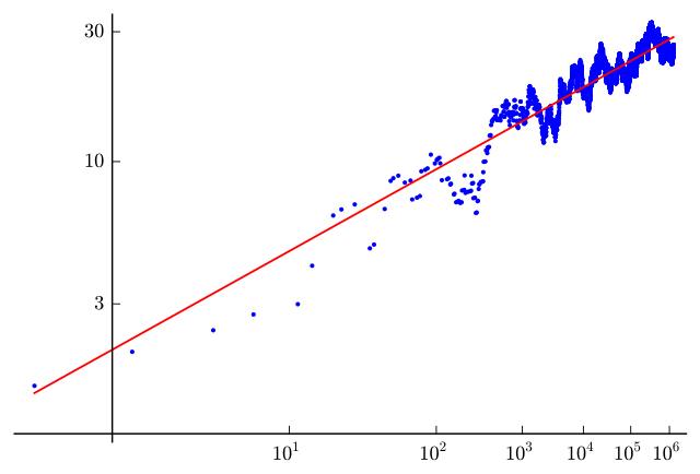
The curve in question is y² = x³ − 5x. This is a curve of rank 1 and one of the curves originally looked at by Birch and Swinnerton-Dyer.

Now, I am a mathematician and not a statistician but even I can see a clear trend and it does seem that the regression line has slope 1 on this plot.

The curve E has rank 1 and when they tried different curves of varying ranks, they found the same pattern every time. The slope of the fitted regression line, it seemed, was always equal to the rank of the curve in question.

More precisely, they stated the bold conjecture that

Here C is some constant.

This computer crunching adventure combined with a great deal of far-sightedness led them to make a general conjecture about the behavior of a curve’s Hasse–Weil L-function L(E, s) at s = 1.

This L-function is defined as follows. Let

and let the discriminant of the curve be denoted Δ. Then we can define the L-function associated with E as the following Euler product

We view this as a function of the complex variable s.

Their conjecture now has the form:

Conjecture (Birch and Swinnerton-Dyer): Let E be any elliptic curve over ℚ. The rank of the abelian group E(ℚ) of rational points of the curve E is equal to the order of the zero of L(E, s) at s = 1.

The reason why it was quite far-sighted is that, at the time, they didn’t even know if a so-called analytic continuation existed for all such L-functions. The problem was that L(E, s) as defined above only converges when Re(s) > 3/2.

That they can all be evaluated at s = 1 by analytic continuation was first proved in 2001 again by using the close connection to modular forms that Andrew Wiles proved.

Sometimes the conjecture is stated using the Taylor expansion of the L-function, but it is saying the same thing in a different way. The field of rational numbers can be replaced by a more general field but I didn’t want to go into more abstraction than necessary.