In the 1960s and '70s, before nonparametric regression methods became widely available, it was common to apply a nonlinear transformation to the dependent variable before fitting a linear regression model. This is still done today, with the most common transformation being a logarithmic transformation of the dependent variable, which fits the linear least squares model log(Y) = X*β + ε, where ε is a vector of independent normally distributed variates. Other popular choices include power transformations of Y, such as the square-root transformation.

The Box-Cox family of transformations (1964) is a popular way to use the data to suggest a transformation for the dependent variable. Some people think of the Box-Cox transformation as a univariate normalizing transformation, and, yes, it can be used that way. (I will discuss the univariate Box-Cox transformation in another article.) However, the primary purpose of the Box-Cox transformation is to transform the dependent variable in a regression model so that the residuals are normally distributed. The Box-Cox transformation attempts to find a new effect W = f(Y) such that the residuals (W - X*β) are normally distributed, where f is a power transformation that is chosen to maximize the normality of the residuals. Recall that normally distributed residuals are useful if you intend to make inferential statements about the parameters in the model, such as confidence intervals and hypothesis tests.

It is important to remember that you are normalizing residuals, not the response variable! Linear regression does not require that the variables themselves be normally distributed.

This article shows how to use the TRANSREG procedure in SAS to compute a Box-Cox transformation of Y so that the least-squares residuals are approximately normally distributed.

The simplest Box-Cox family of transformations

In the simplest case, the Box-Cox family of transformations is given by the following formula:
fλ(y)={(yλ−1)/λlog(y)λ≠0λ=0fλ(y)={(yλ−1)/λλ≠0log⁡(y)λ=0
The objective is to use the data to choose a value of the parameter λ that maximizes the normality of the residuals (fλ(Y) - X*β).

In SAS, you can use PROC TRANSREG to perform a regression that includes the BOXCOX transformation.

Before performing a Box-Cox transformation, let's demonstrate why it might be necessary. The following call to PROC GLM in SAS performs a least squares regression of the MPG_Highway variable (response) onto two explanatory variables (Weight and Wheelbase) for vehicles in the Sashelp.Cars data set. The residuals from the model are examined in a histogram and in a Q-Q plot:

%let dsName = Sashelp.Cars;
%let XName = Weight Wheelbase;
%let YName = MPG_Highway;
 
proc glm data=&dsName plots=diagnostics(unpack);
   model &YName = &XName;
   ods select ResidualHistogram QQPlot;
quit;

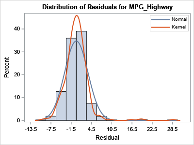
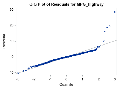
The graphs show that the distribution of the residuals for this model deviates from normality in the right tail. Apparently, there are outliers (large residuals) in the data. One way to handle this is to increase the complexity of the model by adding additional effects. Another way to handle it is to transform the dependent variable so that the relationship between variables is more linear. The Box-Cox method is one way to choose a transformation.

To implement the Box-Cox transformation of the dependent variable, use the following syntax in the TRANSREG procedure in SAS:

• On the MODEL statement, enclose the name of the dependent variable in a BOXCOX transformation option.
• After the name of the dependent variable, you can include options for the transformation. These options determine which values of the parameter λ are used for the transformation. I typically use the values LAMBDA=-2 to 2 by 0.1, although sometimes I will use -3 to 3 by 0.1.
• I like to use the CONVENIENT option, which tells PROC TRANSREG to use simpler transformations, when possible, instead of the mathematically optional transformation. The idea is that if the optimal transformation is a value like λ=0.4, you might prefer to use a square-root transformation (λ=0.5) if there is no significant difference between the two parameter values. Similarly, you might prefer a LOG transformation (λ=0) over an inconvenient value such as λ=0.1. The documentation contains details of the CONVENIENT option.

The following call to PROC TRANSREG implements the Box-Cox transformation for these data and saves the residuals to a SAS data set:

proc transreg data=&dsName ss2 details plots=(boxcox);
   model BoxCox(&YName / convenient lambda=-2 to 2 by 0.1) = identity(&XName);
   output out=TransOut residual;
run;

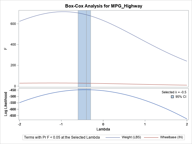
The procedure forms 41 regression models, one for each requester value of λ in the range [-2, 2]. To help you visualize how each value of λ affects the normality of the residuals, the procedure creates the Box-Cox plot, which is shown. The graph is a panel that shows two plots:

• The bottom panel shows the graph of the log-likelihood function (for the normality of the residuals) for each value of λ that was examined. For these data and family of models, the log-likelihood is maximized for λ= -0.4. A blue band shows a confidence interval for the maximal lambda. The confidence interval includes the value -0.5, which is a more "convenient" value because it is related to the transformation y → 1/sqrt(y). Since the CONVENIENT option was specified, λ= -0.5 will be used for the regression model. (Note: The Box-Cox transformation that is used is 2*(1 - 1/sqrt(y)), which is a scaled and shifted version of 1/sqrt(y).)

• The top panel shows the graph of the F statistics for each effect in the model as a function of the λ parameter. For the optimal and the "convenient" values of λ, the F statistics are large (approximately F=700 for the Weight variable and F=30 for the Wheelbase variable), which means that both effects are significant predictors for the transformed dependent variable.

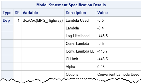
The procedure also displays a table that summarizes the optimal value of λ, the value used for the regression, and other information:

You can use PROC UNIVARIATE to plot the distribution of the residuals for the selected model (λ= -0.5). The name of the residual variable is RYName, where YName is the name of the dependent variable.

proc univariate data=TransOut(keep=R&YName);
   histogram R&YName / normal kernel;
   qqplot R&YName / normal(mu=est sigma=est) grid;
   ods select histogram qqplot GoodnessOfFit Moments;
run;

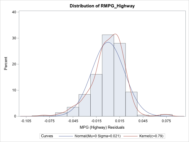
As shown by the histogram of the residuals, the Box-Cox transformation has eliminated the extreme outliers and improved the fit. Be aware that "improving the normality of the residuals" does not mean that the residuals are perfectly normal, especially if you use the CONVENIENT option. A test for normality (not shown) rejects the hypothesis of normality. However, the inferential statistics for linear regression are generally robust to mild departures from normality.

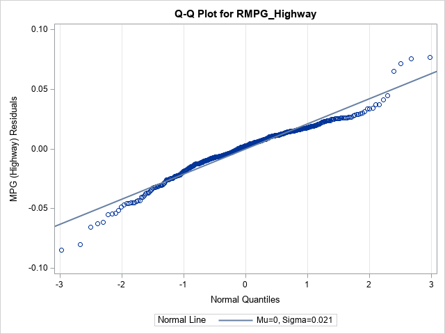
A normal quantile-quantile (Q-Q) plot provides an alternate way to visualize normality. The histogram appears to be slightly left-skewed. In a Q-Q plot, a left-skewed distribution will have a curved appearance, as follows:

The full Box-Cox distribution

There are two mathematical issues with the simple Box-Cox family of transformations:

• Every element of Y must be positive, otherwise, the transformation is not well-defined. A common way to address this issue is to shift the Y variable (if necessary) by a constant, c, so that Y+c is strictly positive. One choice for c is c = 1 - min(Y).
• The magnitude of the transformed variable depends on the parameter λ. This makes it hard to compare regression statistics for different values of λ. Spitzer (1982) popularized using the geometric mean of the response to standardize the transformations so that they are easier to compare. Accordingly, you will often see the geometric mean incorporated into the Box-Cox transformation.

Thus, the general formulation of the Box-Cox transformation incorporates two additional terms: a shift parameter and a scaling parameter. If any of the response values are not positive, you must add a constant, c. (Sometimes c is also used when Y is very large.) The scaling parameter is a power of the geometric mean of Y. The full Box-Cox transformation is
fλ(y)={((y+c)λ−1)/(λg)log(y+c)/gλ≠0λ=0fλ(y)={((y+c)λ−1)/(λg)λ≠0log⁡(y+c)/gλ=0
where g=Gλ−1g=Gλ−1, and G is the geometric mean of Y.

Although the response variable in this example is already positive, the following program uses a PROC SQL calculation to compute the shift parameter c = 1 - min(Y) and write the value to a macro variable. You can then use the PARAMETER= option in the BOXCOX transformation to specify the shift parameter. The geometric mean is much simpler to specify: merely use the GEOMETRICMEAN option. Thus, the following statements implement the full Box-Cox transformation in SAS:

/* use full Box-Cox transformation with c and G. */
/* compute c = 1 - min(Y) and put in a macro variable */
proc sql noprint;                              
 select 1-min(&YName) into :c trimmed from &dsName;
quit;
%put &=c;
 
proc transreg data=&dsName ss2 details plots=(boxcox);
   model BoxCox(&YName / parameter=&c geometricmean 
                         convenient lambda=-2 to 2 by 0.05) = identity(&XName);
   output out=TransOut residual;
run;

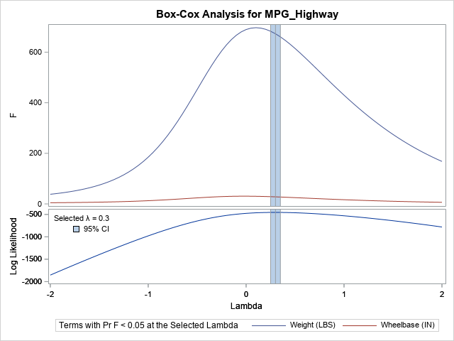
For these data, the value of the c parameter is -11, so when we add c, we are shifting the response variable to the left. For variables that have negative values (the usual situation in which you would use c), you shift the response to the right. The geometric mean scales each transformation. The bottom plot in the panel indicates that λ = 0.3 is the value of λ that makes the residuals most normal. For this analysis, λ = 0.25 is NOT in the confidence interval for λ, so no "convenient" parameter value is used. Instead, the chosen transformation is 0.3.

If you want to examine the distribution of the residuals, you can use the following call to PROC UNIVARIATE:

/* optional: plot the distribution of the residuals */
proc univariate data=TransOut(keep=R&YName);
   histogram R&YName / normal kernel;
   qqplot R&YName / normal(mu=est sigma=est) grid;
   ods select histogram qqplot;
run;

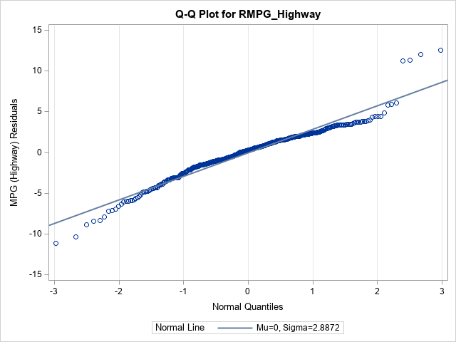
Both the histogram (not shown) and the Q-Q plot indicate that the residuals are approximately normal but are left-skewed.

Advantages and disadvantages of the Box-Cox transformation

The advantage of the Box-Cox transformation is that it provides an automated way to transform a dependent variable in a regression model so that the residuals for the model are as normal as possible. The transformations are all power transformations, and the logarithmic transformation is a limiting case that is also included.

The Box-Cox transformation also has several disadvantages:

• The Box-Cox transformation cannot correct for a poor model, and it might obscure the fact that the model is a poor fit.
• The Box-Cox transformation can be hard to interpret. Similarly, it can be hard to explain to a client. The client asked you to predict a variable Y. Instead, you show them a model that predicts a variable defined as W=((Y+c)λ−1)/(λGλ−1)W=((Y+c)λ−1)/(λGλ−1), where λ= -0.3 and G is the geometric mean of Y. You can, of course, invert the transformation, but it is messy.

Modern nonparametric regression methods (such as splines and loess curves) might provide a better fit. However, I suggest looking at the Box-Cox transformation to see if the method suggests a simple transformation, such as the inverse, log, square-root, or quadratic transformations (λ = -1, 0, 0.5, 2). If so, you can choose the parametric approach for the transformed response.

Summary

This article shows how to use PROC TRANSREG in SAS to perform a Box-Cox transformation of the response variable in a regression model. The procedure examines a family of power transformations indexed by a parameter, λ. For each value of λ, the procedure transforms the response variable and computes a regression model. The optimal parameter is the one for which the distribution of the residuals is "most normal," as measured by a maximum likelihood computation. You can use the CONVENIENT option to specify that a nearby simple transformation (for example, a square-root transformation) is preferable to a less intuitive transformation.

This article assumes that there is one or more regressors in the model. The TRANSREG procedure can also perform a univariate Box-Cox transformation. The univariate case is discussed in a second article.

Further Reading

• Hallahan, Charles, 1990, "A Macro for the Box-Cox Transformation: Estimation and Testing," Proceedings of the Fifteenth Annual SAS Users Group International Conference.
• LaLonde, Steven M., 2012, "Transforming Variables for Normality and Linearity," Proceedings of the 2012 SAS Global Forum.
• SAS Institute, 2020, "Box-Cox Transformations," in the chapter "The TRANSREG Procedure" in the SAS/STAT 15.2 Users Guide.
• Spitzer, J., 1982, "A Primer on Box-Cox Estimation," The Review of Economics and Statistics, pp. 307-313.