The use of Convolutional Neural Networks (CNNs) is widespread. The introduction of deep architectures for feature learning and classification has resulted in a dramatic increase in the performance of visual recognition systems in the past five years. The use of CNNs has achieved remarkable results in a number of fields, including automatic speech recognition, computer vision, language translation, and self-driving cars. CNNs have almost unlimited applications.

DeepMind (from Google) recently published WaveNet, which uses a CNN to generate speech that mimics any human voice (https://deepmind.com/blog/wavenet-generative-model-raw-audio/).

We will discuss the following topics in this article:

• The history of CNNs

• An overview of CNN

• Augmentation of images

History of CNNs

The recognition of pictures by machines has been attempted numerous times over the past few decades. In computers, mimicking the human brain’s visual recognition system is a challenge. Among all the brain’s sensory cognitive systems, human vision is the most complex and hard to mimic. The primary visual cortex, which contains biological neurons, will not be discussed here, but rather artificial neurons will. Images of physical objects are two dimensional, whereas the objects themselves are three dimensional. Our approach to neural networks in this article avoids the use of brain analogies. Known as the father of computer vision, Larry Roberts describes how to extract geometrical information from 2D perspective views of blocks in his 1963 dissertation BLOCK WORLD, which was the first to apply computer vision to geometrical information. Human beings can recognize blocks despite any changes in lighting or orientation that may take place. Computer vision was studied in the context of BLOCK WORLD by many researchers worldwide studying machine learning and artificial intelligence. Throughout his dissertation, he emphasizes the importance of understanding simple edge-like shapes in images. For the computer to understand that these two blocks are the same regardless of orientation, he extracted these edge-like shapes from the blocks:

A simple structure lays the foundation for the vision. A computer vision model begins with a simple structure. The next important concept comes from David Mark, MIT’s computer vision scientist. Mark wrote a article titled VISION that was very influential. This article is very straightforward. The author explains that images consist of layers. Deep learning architecture is based on these two principles, but they do not specify which mathematical model to use.

From the AI lab at Stanford University came the first visual recognition algorithm in the 1970s, known as the generalized cylinder model. This idea is that all things in the real world are composed of simple shapes, and that all of them are combinations of simple shapes. The Pictorial Structure Model, a model from SRI Inc, was also published at the same time. It retains the same concept as the generalized cylinder model, but the parts are connected by springs, which introduces a notion of variability. In 2006, Fujifilm built the first digital camera to use a visual recognition algorithm.

Convolutional neural networks

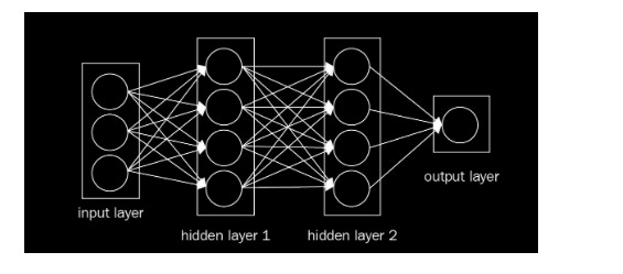
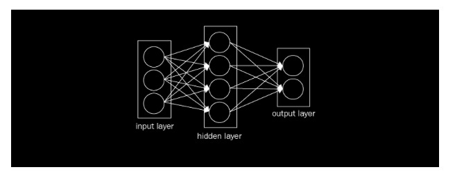
Convolutional neural networks, or CNNs, are quite similar to regular neural networks. However, they still contain neurons that have learned weights as a result of their interactions with data. Dot products are performed by each neuron in response to inputs. However, the last fully connected layer still has a loss function. The nonlinearity function can still be applied. In addition to the tips and techniques that we learned in the previous article, they are still applicable to CNN. The previous article demonstrated that regular neural networks receive input data as a single vector and pass it through a series of hidden layers. The neurons in every hidden layer are fully connected to each other and to the neurons in the previous layer. An individual neuron in a single layer is independent, and it has no connections with another neuron. In the case of image classification, the final layer of fully connected layers contains class scores. A ConvNet consists of three layers in general. Layers 1 and 2 are the convolution layer, layer 3 is the pooling layer, and layer 4 is the fully connected layer. This simple neural network can be seen in the following image:

How does this change? We can encode a few properties into a CNN since it mostly takes images as input, reducing the number of parameters.

Multi-Layer Perceptrons (MLPs) perform better on real-world image data than CNNs. This is due to two factors:

• For feeding an image to an MLP, we converted the input matrix into a simple numeric vector without spatial structure in the last article. The MLP doesn’t understand spatial arrangement. It is for this very reason that CNNs were developed; namely, to uncover patterns within multidimensional data. As opposed to MLPs, CNNs recognize that pixels near each other are more closely related than pixels farther apart: CNN = Input layer + hidden layer + fully connected layer

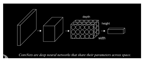
• The types of hidden layers that can be included in CNNs differ from those available in MLPs. ConvNets divide their neurons into three dimensions: width, height, and depth. Each layer uses activation functions to convert its 3D input volume into a 3D output volume of neurons. The red input layer in the following figure, for example, holds the image. Due to its width and height, the image has two dimensions, and its depth is three because it has Red, Green, and Blue channels:

Images are interpreted by computers in what way?

A matrix of pixel values can be used to represent every image. As such, images are functions (f) that map R2 to R.

At position (x, y), f(x, y) represents the intensity value. Usually, the value of the function ranges only between 0 and 255. As with color images, a color image can be viewed as a stack of functions. A color image can include:

As a result, a color image is also a function, but in this case, it does not represent a single number at each (x,y) position. It is instead a vector with three different light intensities, which correspond to three different colors. An image’s details are shown by the following code when input to a computer.

Code for visualizing an image

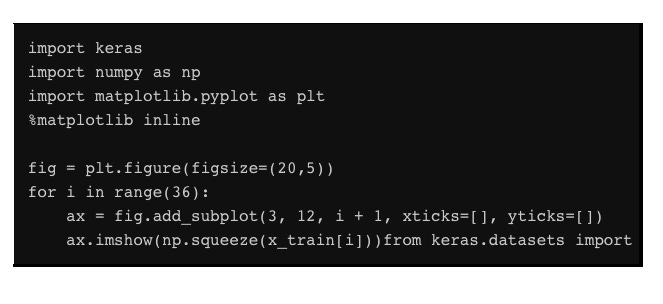
Check out how the following code can be used to visualize an image:

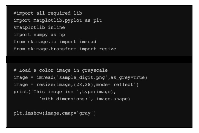
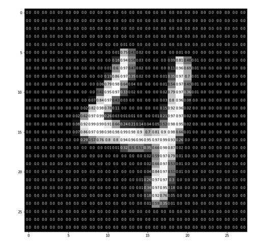
This results in the following image:

In this case, we get the following result:

Using MLPs, we recognized images in the previous article. That approach has two problems:

• The number of parameters is increased

• Vectors are the only inputs, so it flattens a matrix to a vector

We must therefore devise a new method of processing images that retains 2D information. The CNN solves this problem. In addition, CNNs can be fed matrices. This preserves spatial structure. Convolution windows, such as filters or kernels, are defined first, and these are slid over the image.

Dropout

You can think of a neural network as a search problem. In a neural network, each node searches for correlations between the inputs and the correct outputs.

As a result of dropout, nodes are randomly turned off during forward propagation, which prevents weights from convergent to identical positions. Then, all the nodes are switched on, and they back-propagate. The same procedure can be followed to dropout a layer during forward propagation by setting some of its values to zero at random.

Input layer

Image data is stored in the input layer. The input layer has three inputs as shown in the figure below. A fully connected layer consists of neurons in two adjacent layers, which are connected pairwise but don’t share any connections within that layer. Basically, the neurons in this layer have full connectivity with the neurons in the previous layer. Activations of these genes can therefore be calculated using a matrix multiplication, optionally with bias. Fully connected neurons are connected to a global region in the input, while neurons in a convolutional layer are also connected to a local region:

Convolutional layer

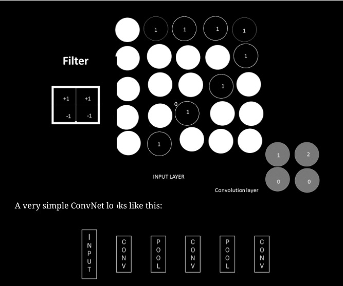
In relation to ConvNet, convolution has the main purpose of extracting features from an image. ConvNet’s computation is mainly performed by this layer. Convolution is not discussed here in detail, but we will understand how it works over images.

CNNs have a lot of use for ReLU activation functions.

Layers of convolution in Keras

Keras requires the following modules to create a convolutional layer:

A convolutional layer can then be created by following the following format:

The following arguments must be passed:

• Filters: How many filters are available.

• Kernel_size: A number that defines both the height and width of the (square) convolution window. Additional optional arguments may also be set.

• Convolution stride: The length of the convolution. When not specified, it defaults to one.

• The padding is either valid or the same. If nothing is specified, the padding is set to valid.

• It is typically relu that activates the system. If no activation is specified, the system does not activate. Each convolutional layer in your network should have a ReLU activation function.

As part of a model, you must provide an additional parameter called input_shape if you want your convolutional layer to appear after the input layer. The input is specified by three tuples (height, width, and depth) in that order.

Convolutional layers can also be controlled by a variety of other tunable arguments, including:

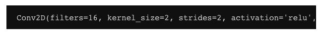
For instance, a CNN can be built with an input layer that accepts images in grayscale that are 200 x 200 pixels. When this occurs, the next layer would be a 16-filter convolutional layer, with width and height equal to 2. Let’s configure the filter so it jumps two pixels together as we go along with the convolution. Therefore, we can build a layer with a convolutional filter that does not pad the images with zeros by implementing the following code:

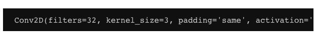
The next layer in our CNN model can be a convolutional layer after we have built a CNN model. In this layer, we will have 32 filters with widths of 3 and heights of 3, which will take the layer from the previous example as their input. While we are doing the convolution, we will set the filter so that it jumps one pixel at a time, so that the convolutional layer can see all regions of the previous layer as well. The following code can be used to create a convolutional layer:

Explanation 3: The convolutional layers in Keras can also be constructed with 64 filters and an activation function of ReLU. The convolution is offered here with a stride of 1 and padding set to valid as well as all other arguments at their default values. The following code can be used to build a convolutional layer:

Pooling layer

In general, a convolutional layer is stacked feature maps, each corresponding to a filter. Convolution becomes more dimensional as more filters are added. More parameters mean a higher dimensionality. By progressively reducing the spatial size of the representation, the pooling layer reduces overfitting by reducing the number of parameters and computations. It is frequently used in conjunction with the convolutional layer. The most common pooling approach is maximum pooling. Other pooling functions, such as average pooling, can also be performed by pooling units. The size of each filter and the number of filters in a CNN determine the behavior of the convolutional layer. As the number of nodes increases in a convolutional layer, so does the size of the pattern, and as the size of the filter increases, the number of filters increases. Additional hyperparameters may also be tuned. Convolution stride is one such parameter. It determines how much the filter slides over an image. Strides of 1 move the filter horizontally and vertically by 1 pixel. In this case, the convolution returns to the same size as the input image’s width and depth. The convolutional layer corresponding to a stride of 2 is half the width and half the height of the image. We can ignore unknown values outside of the image or replace them with zeros if the filter extends outside the image. Padding is the term for this process. Keras allows us to set padding = ‘valid’ if we don’t mind losing a few values. In any case, padding = ‘same’:

Classification of images — a practical example

Detecting regional patterns in an image is made easier with the convolutional layer. Following the convolutional layer, the max pooling layer helps reduce dimensionality. A picture classification example that uses all the principles we studied in the previous sections is given below. Before doing anything else, it’s important to make all images the same size. A second input.shape() parameter is required for the first convolution layer. The following section describes how a CNN can be trained to classify images from the CIFAR-10 database. The CIFAR-10 dataset contains 60,000 32 x 32 color images. Each image is classified into a category with 6,000 images. Airplane, automobile, bird, cat, dog, frog, horse, ship, truck, and so on are the categories. The following code demonstrates how this is done:

Please subscribe to my newsletter and get access to the complete article. By subscribing you can read hundreds of articles, and also find source code with explanations, which you can add to your resume to make it shine. So please consider subscribing. It also helps me pay my tuition fees. Thanks for understanding.